Data-Level Parallelism in Vector, SIMD, and GPU Architectures
- Chapter 4 in Computer Architecture A Quantitative Approach (6th) by Hennessy and Patterson (2017)
Introduction
-
Single instruction multiple data (SIMD) classification was proposed by Flynn, 1966
- A question for the SIMD architecture: How wide a set of applications has significant data-level parallelism (DLP)?
- Matrix-oriented computations of scientific computing
- Media-oriented image
- Sound processing
- Machine learning algorithms
- VS MIMD
- MIMD fetch one instruction per data operation
- SIMD : A single instruction can launch many data operations
- $\rightarrow$ More energy-efficient
- The programmer continues to think sequentially yet achieves parallel speedup by having parallel data operations.
- Three variations of SIMD
-
Vector architectures
- Easier to understand and compile to than other SIMD variations
- Considered too expensive before
- High memory bandwidth,
- Widespread reliance on caches
-
Multimedia SIMD instruction set extensions
- Basically simultaneous parallel data operations
- x86 + MMX (Multimedia extensions) in 1996
- x86 + SSE (Streaming SIMD extensions)
- x86 + AVX (Advanced vector extensions), recently.
-
Graphics processing units (GPUs)
- Comes from graphic accelerator community
- Share features with vector architectures
- Strong ecosystem
- GPU system
- System processor + system memory + GPU + GPU-memory
- a.k.a. heterogeneous architecture
-
Vector architectures
- The goal of this chapter
- Understand why vector is more general than multimedia SIMD
- Understand the similarities and differences between vector and GPU architectures
Vector Architecture
The most efficient way to execute a vectorizable application is a vector processor.
- Jim Smith, ISCA 1994
- Motivation
- Deliver good performance
-
Without OoO superscalar processors
- $\rightarrow$ High complexity and expensive energy consumption
- With simple in-order scalar processors
- Steps in vector architectures (VA)
- (1) Grab sets of data elements scattered about memory
- (2) Place them into large sequential register files
- (3) Operate on data in those register files
- (4) Disperse the results back into memory
- A single instructions in VA
- Works on vectors of data
- Dozens of register-register operation on independent elements
-
Large register files
- Act as compiler-controlled buffers
- Hide memory latency
- Use deep pipeline for vector load/store
- Pay long latency only once per vector load/store
- Amortize the latency over, say, 32 elements
- Leverage memory bandwidth
- Keep the memory busy for contiguous data fetching invoked by a single vector load/store
RV64V Extension
- Loosely based on the 40-year-old Cray-1
- At the time of this edition, RVV (RISC-V Vector extension) was still under development (version 0.7xx)
- RV64V = RISC-V base instructions plus the vector extension
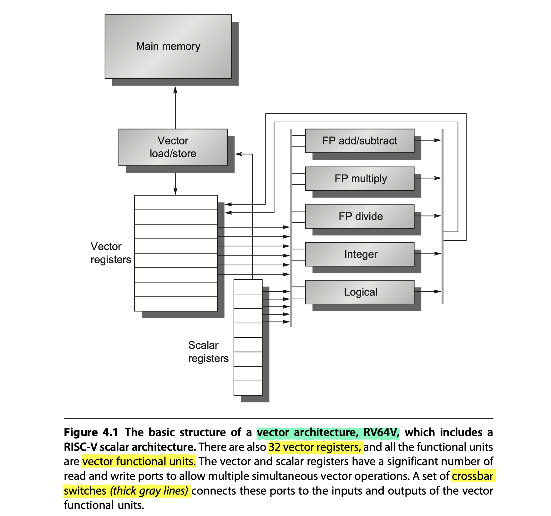
The primary components of RV64V?
-
Vector registers
- Each vector register holds a single vector
- 32 64-bit registors in RV64V
- Register file (RF) $\rightarrow$ Enough ports to feed all the vector functional unit (VFU)
- At least 16 read ports, 8 write ports
- Connected to the functional unit input/outputs via two crossbar switches
- Need high bandwidth? $\rightarrow$ Multiple banks that works well with long vector
-
Vector functional units (VFUs)
- Fully pipelined $\rightarrow$ Start a new operation on every clock cycle
- Control unit
- Detect hazards
- Structural hazards from FUs
- Data hazards on register accesses
-
Vector load/store units
- Loads or stores a vector to or from memory
- Fully pipelined
- After an initial latency,
- Move words between vector registers and memory
- With a bandwidth of one word per clock cycle
- Also handle scalar load/store
-
A set of scalar registers
- Normal 31 general-purpose registers, 32 floating-point registers of RV64G
- Provide data, addresses
- One input of VFUs latches scalar values
-
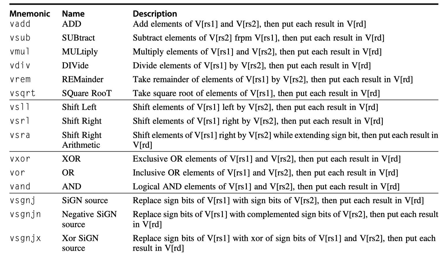
RV64V vector instructions
- Suffix
.vv= Both operands are vectors - Suffix
.vs= 1st/2nd operand is vector/scalar - Suffix
.sv= 1st/2nd operand is scalar/vector - eg.
vsub.vv,vsub.vs,vsub.sv - Assembler $\rightarrow$ Supply the appropriate suffix
- The VFU gets a copy of the scalar value at instruction issue time
-
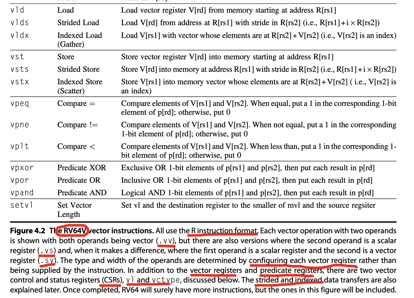
vld/vst- Vector load/store
- One operand = Vector register to be loaded or store
- The other operand = RV64G general-purpose register with the starting address of a vector
- Suffix
-
Dynamic register typing
- Varying data sizes (Kozyrakis and Patterson, 2002)
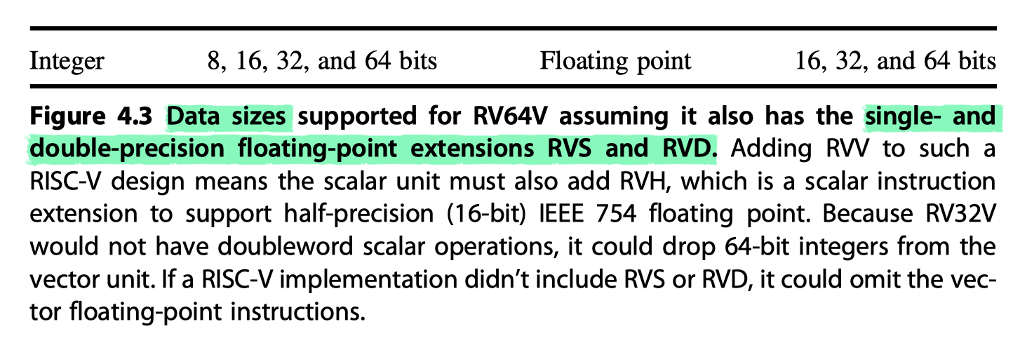
- Note that Figure 4.2 omit the data type and size!
- RVV associates the data type and data size with each vector register
- A program configures the vector registers being used to specify their data type and widths $\rightarrow$ See the options for RV64V in Figure 4.3
- 32 64-bit elements = 128 $\times$ 16-bit elements = 256 $\times$ 8-bit elements
- So, useful for both multimedia (low precision) and scientific application (high precision)
-
Benefit of dynamic register typing
- Reduces the number of instruction types
- Lets programs disable unused vector registers
- eg. 1024 bytes of vector memory = 4 vector registers enabled $\times$ 64-bit float $\times$ 32 elements per register (i.e. maximum vector length ($mvl$), set by the processor, not by software)
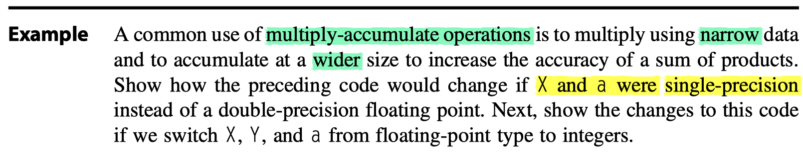
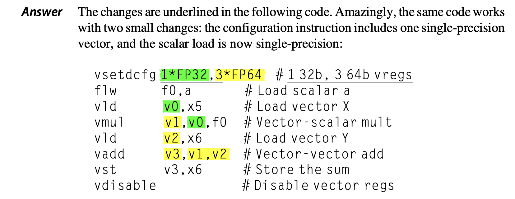
- Implicit conversion between different size operands (No need of additional explicit conversion instructions)
-
Complaint on the vector architecture’s larger state
- Slower context switch time (to save and load the large states)
- Our implementation of RV64V
- Increases state a factor of 3
- From 2 $\times$ 32 $\times$ 8 = 512 bytes to 2 $\times$ 32 $\times$ 24 = 1536 bytes
- A pleasant side effect of dynamic register typing: The program can configure vector registers as disabled when they are not being used, so no need to save and restore them on a context switch
-
Additional registers
-
vl- Vector length register
- Used when the natural vector length $!=$
mvl
-
vctype- Records register types
-
p_i- Predicate registers
- Used when loops involve IF statements
-
CSRs- Control and status registers
-
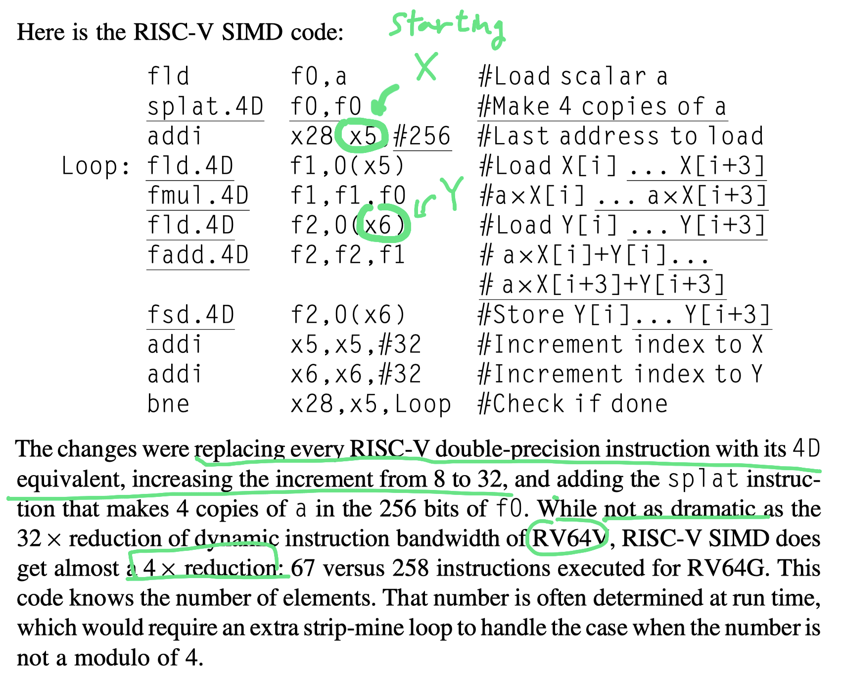
How Vector Processors Work: An Example
- Look at a vector loop for RV64V
- $Y=a \times X + Y$
- SAXPY or DAXPY
- S: Single precision
- D: Double precision
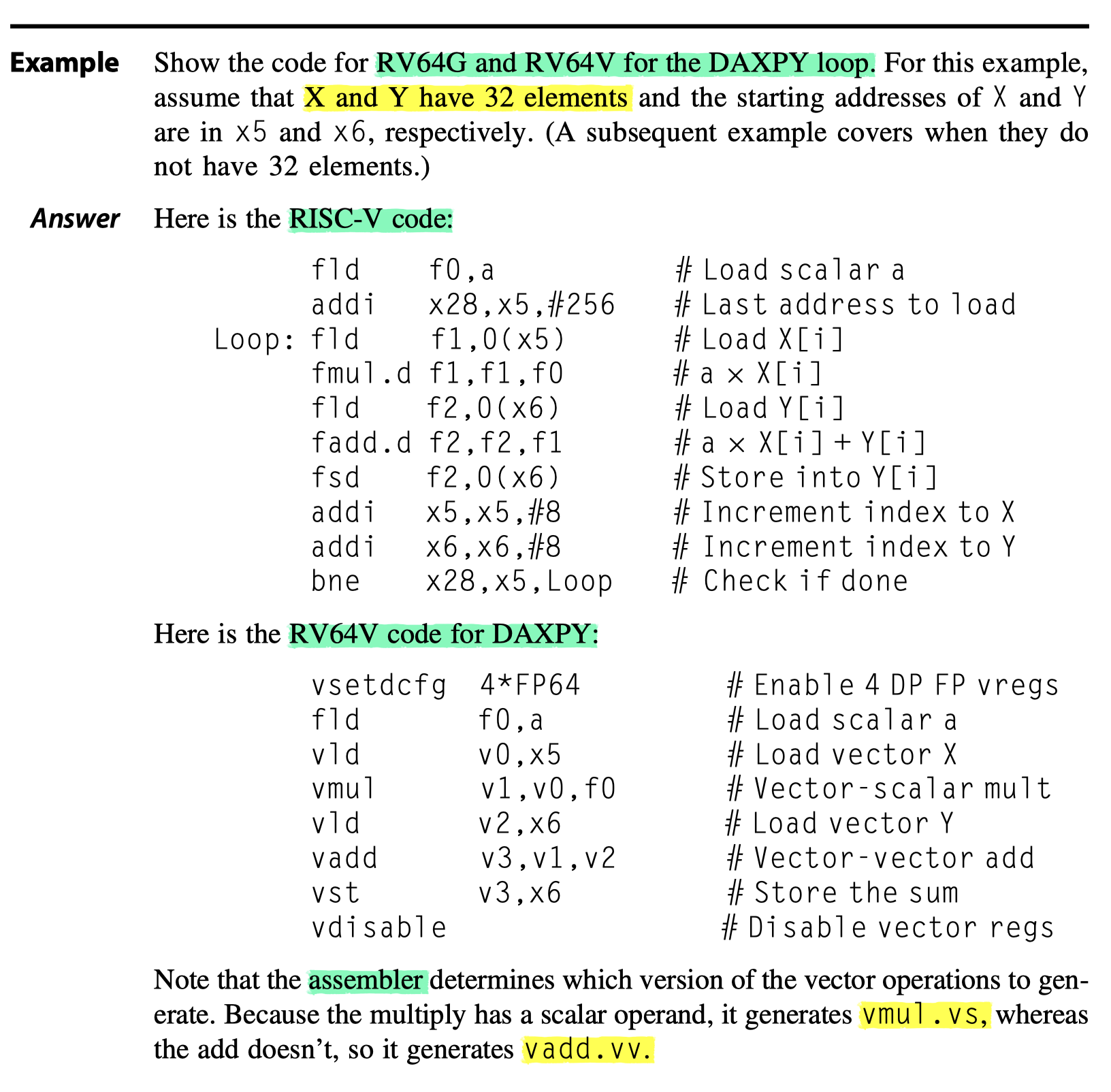
-
vsetdcfg- Initialize the RF configuration
- eg. Four vector registers to hold 64-bit FP data
-
vdisable- Disable all vector registers
- If context switch after
vdisable? $\rightarrow$ No additional state to save
- Vectorizability
- A code is vectorizable/vectorized when …
- No dependences between iterations of a loop
- i.e. No loop-carried dependences
-
Key advantage of RV64V compared to RV64G?
- Greatly reduces the dynamic instruction bandwidth
- Only 8 instructions for RV64V vs 258 for RV64G
- Greatly reduces frequency of pipeline interlocks
- RV64G: Every
fadd.dmust wait for afmul.dandfsd, 32$\times$ more stalls than RV64V - RV64V: Stall only for the first element in each vector by using chaining
-
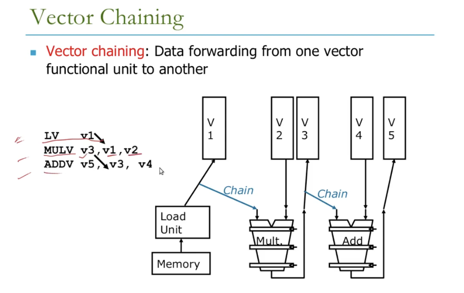
Chaining?
- Forwarding of element-dependent operations
- Dependent operations are “chained” together
- eg. Adjacent
vmulandvaddare dependent, but only the first element’s stall is required
- Stall only once per vector instruction rather than once per vector element!
- RV64G: Every
- Greatly reduces the dynamic instruction bandwidth
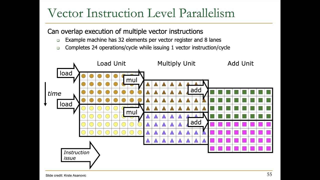
Vector Execution Time
- Three factors for the execution time
- Length of the operand vectors
- Structural hazards among the operations
- Data dependences
-
Vector functional units
- Multiple parallel pipelines (or lanes)
- Produce two or more results per clock cycles $\rightarrow$ Initiation rate
- The rate at which a vector unit consumes new operands and produces new results
- May have VFUs that are not fully pipelined
-
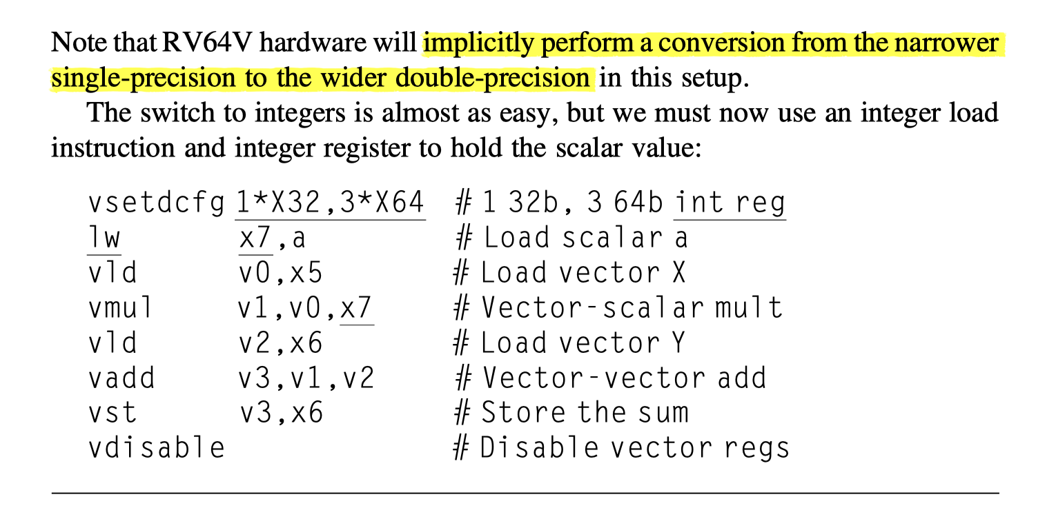
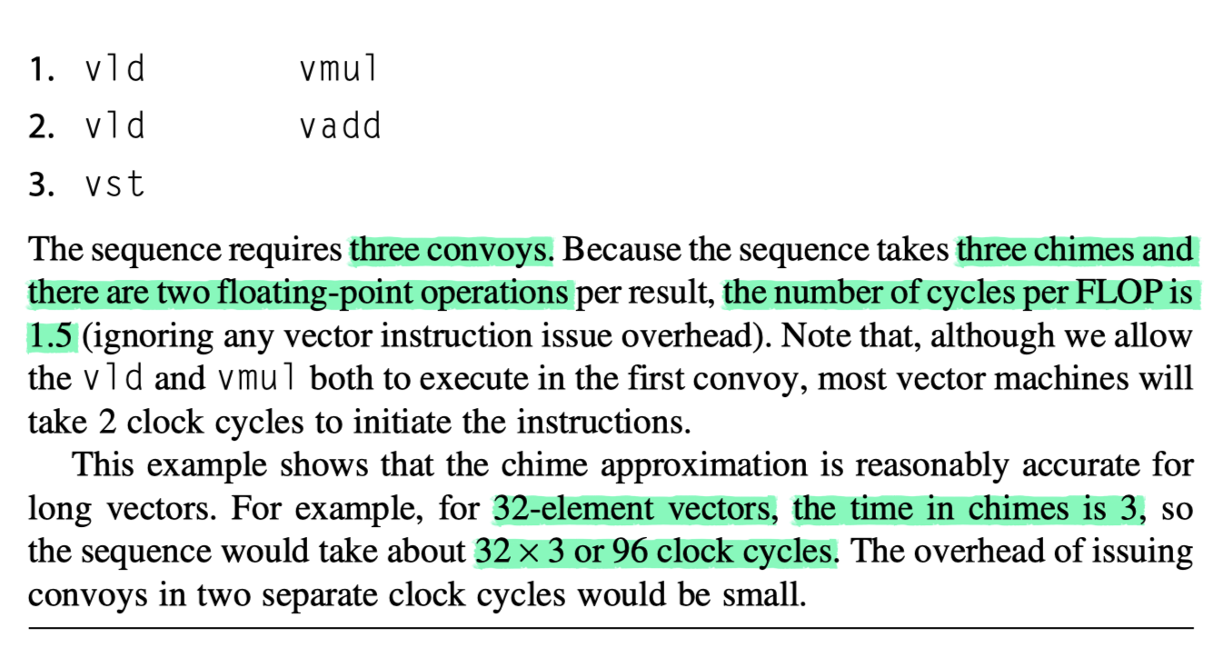
Convoy
- The set of vector instructions that
- Could potentially execute together.
- The instructions in a convoy must not contain any structural hazards
- If $\exists$ (structural hazards) $\rightarrow$ Serialized and initiated in different convoys
- eg.
vld+vmulin the same convoy
- Counting #Convoy $\rightarrow$ Performance estimation
- Instructions with RAW hazard in the same convoy?
- No problem!
-
Chaining allows them to be in a same convoy
- The results from the first functional unit in the chain are “forwarded” to the second functional unit
-
Chaining implementation
- Allowing the processor read and write a particular vector register at the same time, albeit to different elements
- Early version:
- Worked just like forwarding in scalar pipelining
- Restricted the timing
- Recent version:
- Flexible chaining
- Allows a vector instruction to chain to essentially any other active vector instruction, assuming that we don’t generate a structural hazard.
- Estimate the execution time of a convoy?
-
Chime:
- A metric to estimate the length of a convoy
- Simply the unit of time taken to execute one convoy
- $m$ convoys executes in $m$ chimes
- Vector length of $n$ $\rightarrow$ Approximately, $m\times n$ clock cycles for our simple RV64V implementation
- Measuring time in chimes $\rightarrow$ Better approximation for long vectors than for short ones
- The length of vectors is typically much greater than the number of instructions in the convoy $\rightarrow$ we will simply assume that the convoy executes in one chime.
-
Chime:
- Sources of overhead ignored by the chime model
- (1) Vector instruction issue overhead
- (2) Vector start-up time
- Most important source of overhead
- Pipelining latency of the VFU
- eg. 6 clock cycles for FP add, 7 for FP multiply, 20 for FP divide, 12 for vector load
- Questions for optimization of vector architectures
- How can a vector processor execute a single vector faster than one element per clock cycle?
- Multiple elements per clock cycle improve performance.
- How does a vector processor handle programs where the vector lengths are not the same as the maximum vector length (mvl)?
- Because most application vectors don’t match the architecture vector length, we need an efficient solution to this common case.
- What happens when there is an IF statement inside the code to be vectorized?
- More code can vectorize if we can efficiently handle conditional statements.
- What does a vector processor need from the memory system?
- Without sufficient memory bandwidth, vector execution can be futile.
- How does a vector processor handle multiple dimensional matrices?
- This popular data structure must vectorize for vector architectures to do well.
- How does a vector processor handle sparse matrices?
- This popular data structure must vectorize also.
- How do you program a vector computer?
- Architectural innovations that are a mismatch to programming languages and their compilers may not get widespread use.
- How can a vector processor execute a single vector faster than one element per clock cycle?
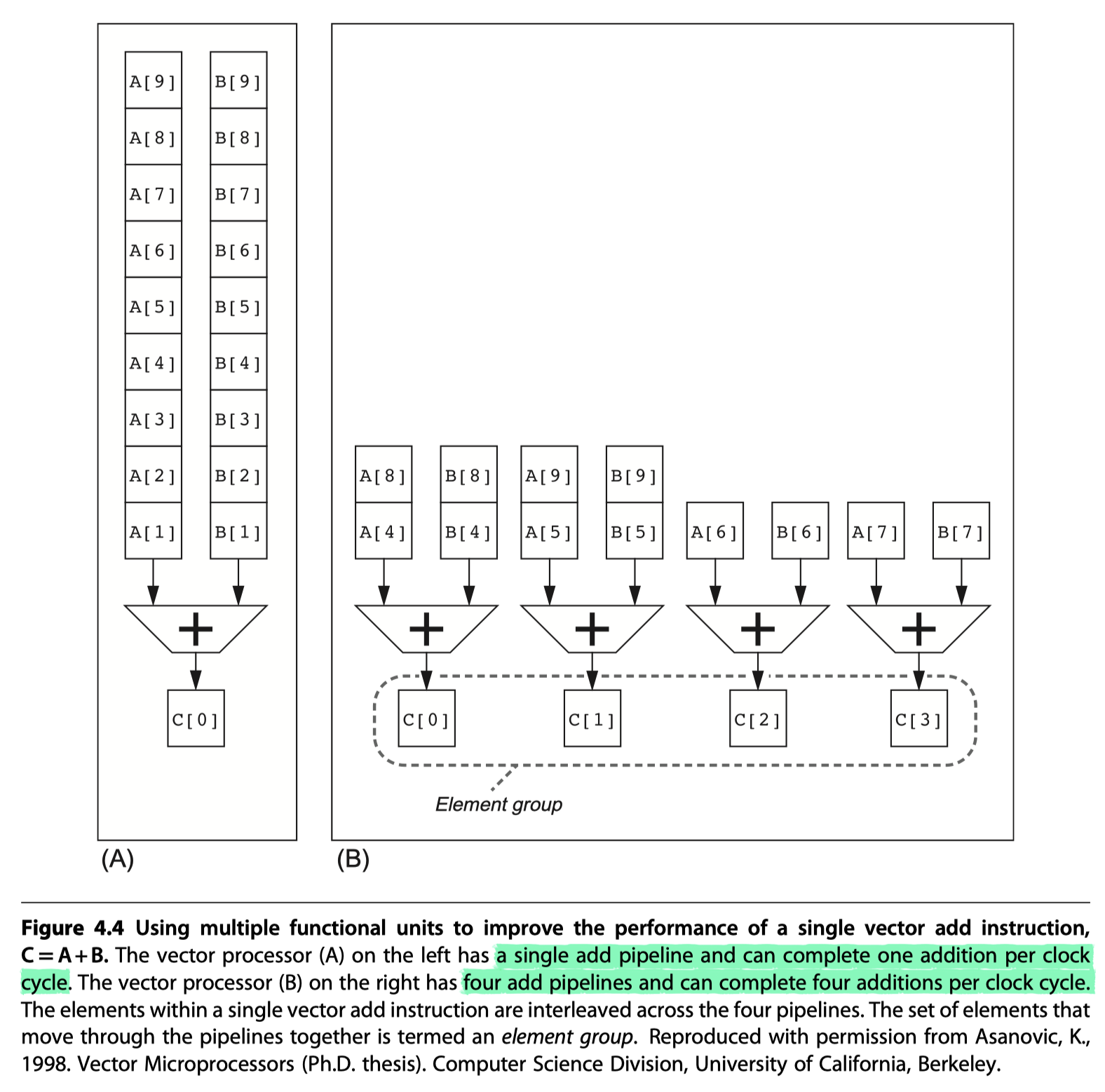
Multiple Lanes: Beyond One Element per Clock Cycle
- Figure 4.4: How to improve vector performance by using parallel pipelines to execute a vector add instruction
- Interleave the elements within a single vector instruction
- ==Multiple parallel lanes
- Run out of instruction bandwidth?
- ILP techniques to supply enough vector instructions
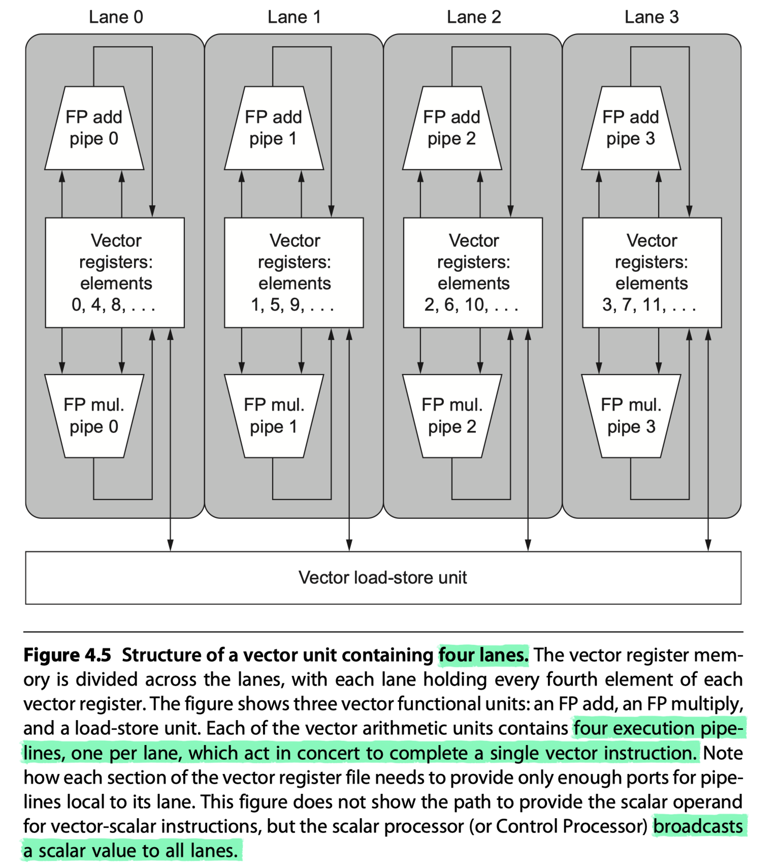
- Figure 4.5: The structure of a four-lane vector unit
- #clocks for a chime: 32 cycles $\rightarrow$ 8 cycles
- Each lane $\ni$ One portion of the VRF, one execution pipeline from each VFU
- Each VFU executes vector instructions @ one element group per cycle, one per lane
- The first lane holds the first element (element 0) for all vector registers
- The arithmetic pipeline = local to the lane without communicating with other lanes
- Adding multiple lanes
- Little increase in control complexity
- No change to existing machine code
- Allows to trade off die area, clock rate, voltage, energy
- Halving clock rate + Doubling #lanes = Same peak performance
Vector-Length Registers: Handling Loops Not Equal to 32
- Maximum vector length (mvl)
- Natural vector length
- Unlikely to match the real vector length in a program
- Real program’s length of a particular vector operation $\rightarrow$ Unknown at compile time
1
2
3
4

// n : Unknonwn in compile time
for (i = 0; i < n; i=i+1){
	Y[i] = a*X[i] + Y[i];
}
- Vector-length registers (
vl)-
vlcontrols the length of any vector operation -
vl$\leq$mvl - Then, the length of vector registers can be later decided without changing the instruction set
- Multimedia SIMD extensions
- No equivalent of
mvl$\rightarrow$ Expand the instruction set for each vector length
- No equivalent of
-
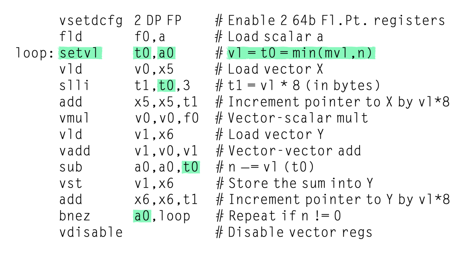
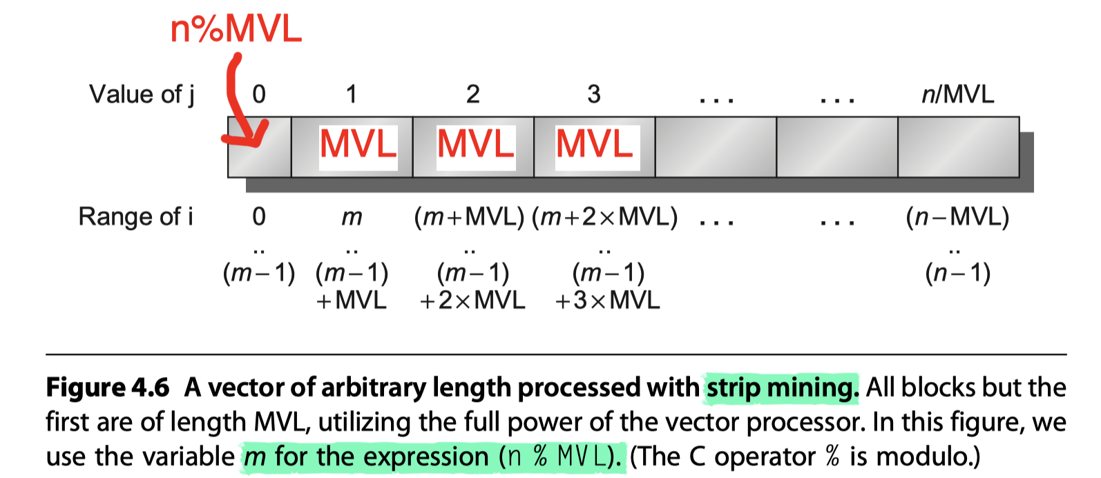
- What if vector length >
mvl?- Just do strip mining
- i.e. The generation of code such that each vector operation is done for a size less than or equal to the
mvl. - One loop = Multiple of
mvl+ another loop for any remaining iterations $\leq$mvl - RISC-V’s
setvlinstruction- Writes the smaller of the
mvland the loop variablen(i.e. min(mvl,n)) intovlregister - Also writes another scalar register to help with later loop bookkeeping
- Writes the smaller of the
Predicate Registers: Handling IF Statements in Vector Loops
- Two main reasons for lower levels of vectorization?
- IF statements inside loops
- Use of sparse matrices
1
2
3
4
5

for (i = 0; i < 64; i=i+1){
	if (X[i] != 0){
		X[i] = X[i] – Y[i];
	}
}
- How to vectorize?
- Use vector-mask control
- Predicate registers in RV64V
- Hold the mask (Boolean vector)
- Provide conditional execution
- Similar to Boolean condition in scalar instruction
- The predicate registers
p0is set- Vector instructions only operate on the vector elements whose corresponding entries in
p01.==
- Vector instructions only operate on the vector elements whose corresponding entries in
-
With the starting addresses of X and Y are in
X5andX6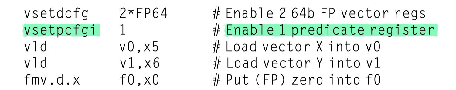
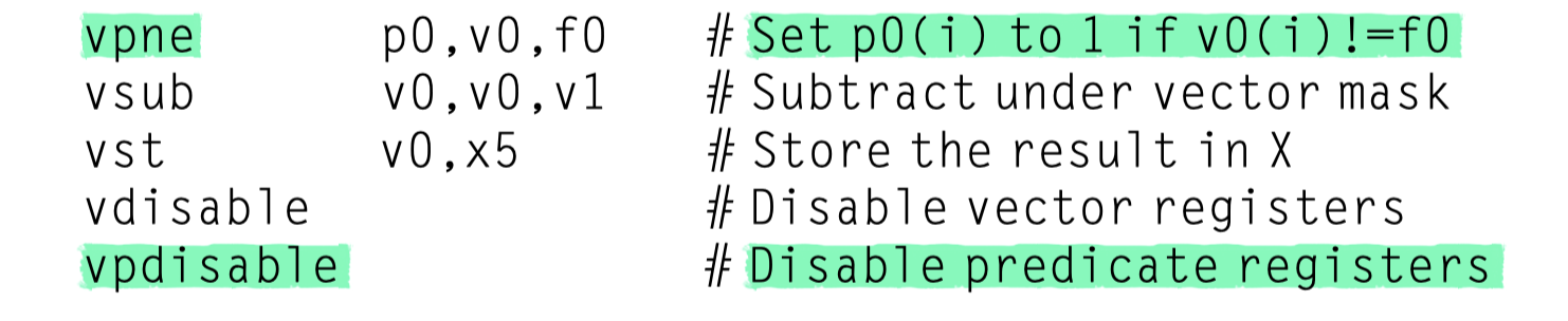
- Compiler writes use the term IF-conversion
- Transform an IF statement into a straight-line code sequence using conditional execution with vector-mask control.
- Difference with GPUs for handling conditional statements
- Vector processors:
- Make predicate registers part of the architectural state
- Rely on compilers to manipulate mask registers explicitly
- GPUs:
- Same effect using hardware
- Manipulate internal mask registers that is invisible to GPU software
- Both spends the time to execute vector element depending on mask bits (0 or 1)
- Vector processors:
Memory Banks: Supplying Bandwidth for Vector Load/Store Units
- Start-up time for a load
- Time to get the first word from memory into a register
- Over 100 clock cycles on many processors
- Reduce penalty?
- Use cache
- Here, assume 12 clock cycles like Cray-1
- Initiation rate for a load
- No stall? $\rightarrow$ Rate at which new words are fetched or stored
- Stall? $\rightarrow$ May be less then 1 clock cycle
- Maintain one word per one cycle?
- Spread accesses across multiple independent memory banks
- Why several independent access rather then the simple memory interleaving ?
- Support simultaneous access from multiple loads or stores
- Support the ability to load/store data words that are not sequential
- Shared memory $\rightarrow$ Each processor generates its own separate stream of addressses
-
So, a larger number of independent memory banks is desired!
- Example: Cray T932’s memory banks
- 32 processors with max 4 loads/2stores per cycle
- Processor cycle = 2.167ns
- SRAM cycle = 15ns
- Minimum memory banks?
- 32x6 = 192 memory reference per clock cycle
- One memory access takes 15ns/2.167ns = 6.92 ~ 7 processor-clock-cycles
- 192 accesses x 7 processor-clock-cycles = 1344 memory banks !!
- Cray T932 = 1024 memory banks
- Not full bandwidth supprort
Stride: Handling Multidimensional Arrays in Vector Architectures
- The position of adjacent elements in a vector may not be sequential!
1
2
3
4
5
6
7

// GEMM A = A + BxD
for (i = 0; i < 100; i=i+1)
	for (j = 0; j < 100; j=j+1) {
		A[i][j] = 0.0;
		for (k = 0; k < 100; k=k+1)
			A[i][j] = A[i][j] + B[i][k] * D[k][j];
}
- In the GEMM code for A = A + B $\times$ D operation,
- (Each element of A) += (Each row of B) $\times$ (Each column of D)
- So, want to …
- vectorize each row of B and each column of D
- Strip-mine the most inner loop with k
- Matrix allocation
- Row major in C
- Column major in Fortran
- Either the elements in the row or the elements in the column are not adjacent in memory
- Elements in column vectors of D matrix $\rightarrow$ Separated by the row size (100) times 8 (double type’s #bytes) !!
- Stride
- Distance separating elements to be gathered into a single vector register
- B’s unit stride = 1 double word (8 bytes)
- D’s non-unit stride = 100 double words (800 bytes)
- D column vector stored in a vector register? $\rightarrow$ Elements become adjacent
- Stride computation
- 800 bytes = the row size (100) $\times$ 8 (double type’s #bytes)
- Compute dynamically because of not knowing at the compile time
- Vector stride can be put in a general-purpose register
- Like the vector starting address
-
VLDS/VSTS: Load/store vector with stride- Fetches the vector with non-unit stride to vector register
- Complication of the memory system due to non-unit stride
- Possible to request accesses from the same bank frequently
- The worst possible stride
- = A multiple of #memory banks
- Every access to memory will collide with the previous access
- Need to wait for bank busy time (eg. 6 cycles)
- Memory bank conflict occurs when …

- Example of bank conflict
- 8 memory banks
- 6 clocks of bank busy time
- 12 cycles of memory latency
- 64-element vector load with stride of 1? and 32?
- Stride of 1 : 12 + 64 = 76 cycles
- 1.2 clock cycles per element
- Stride of 32 :
- 12 (latency) + 1 + 6 $\times$ 63 = 391 cycles
- 6.1 clock cycles per element
- Stride of 1 : 12 + 64 = 76 cycles
Strided Accesses and TLB Misses in Cross-Cutting Issues
- How they interact with TLB for virtual memory ?
- In vector architectures or GPUs
- Possible to get one TLB miss for every access to an element in the array!
- The same type of collision can happen with caches, but the performance impact is probably less.
Gather-Scatter: Handling Sparse Matrices in Vector Architectures
-
Execute sparse matrix operations in vector mode?
-
Sparse matrices
- Stored in some compacted form
- Accessed indirectly
1
2
3
4
5
6
// Sparse vector sum
for (i = 0; i < n; i=i+1){
// Elements of sparse matrices A and B are
// Accessed indirectly via K and M index vectors
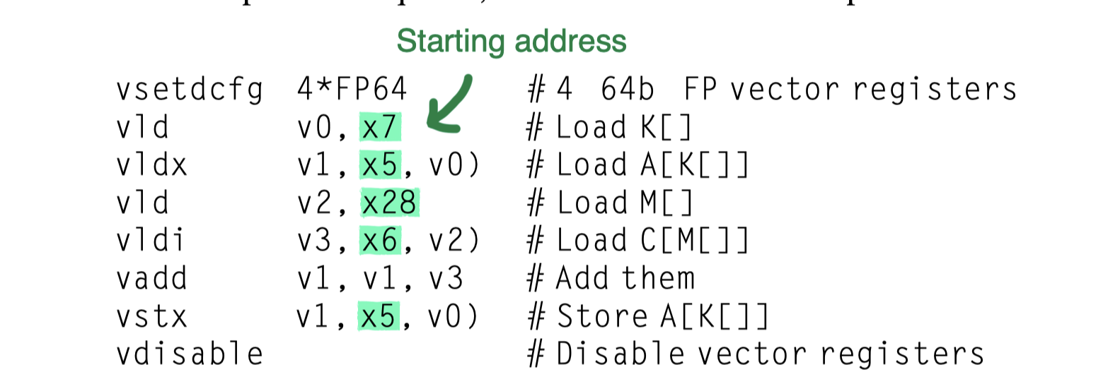
A[K[i]] = A[K[i]] + C[M[i]];
}
- Gather-scatter operations using index vectors
- Support moving between
- Compressed representation
- $\leftrightarrow$ Normal representation
- Gather operation
- Takes an index vector
- Fetches the vector
- Whose elements are at the addresses given by adding a base address to the offsets given in the index vector
- $\rightarrow$ Dense vector in a vector register
- Scatter store
- Using the same index vector
- Store the sparse vector in an expanded form
- Slower access than non-indexed load/store
- Memory banks are not know from the start of the instruction
- Register file must also provide communication between the lanes of a vector unit to support gather and scatter
- Possible conflicts at many places
- Refer to Section 4.7 for memory system with better performance
- Support moving between
- Gather-scatter in RV64V
-
vldi: Load vector indexed or gather -
vsti: Store vector indexed or scatter
-
- On programming model
- A simple vectorizing compiler could not automatically vectorize the preceding source code
- Because the compiler would not know that the elements of K are distinct values, and thus that no dependences exist.
- Instead, a programmer directive would tell the compiler that it was safe to run the loop in vector mode.
- VS GPUs
- All loads are gathers in GPUs
- All stores are scatters in GPUs
- i.e. No separate instructions restrict addresses to be sequential
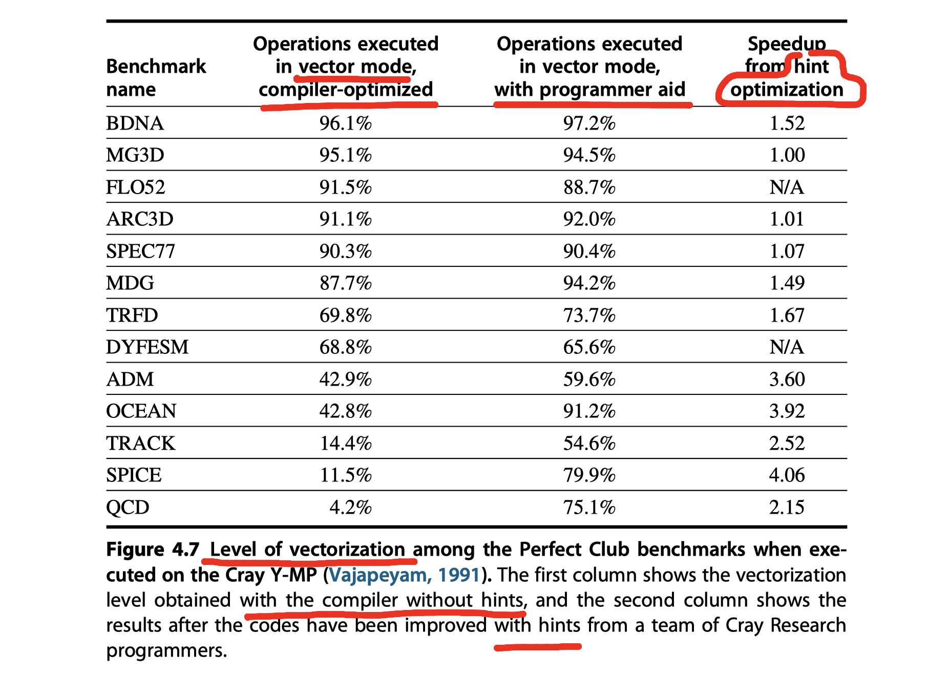
Programming Vector Architectures
- An advantage of vector architectures is that
- Compilers can tell programmers at compile time
- Whether a section of code will vectorize or not,
- Often giving hints as to why it did not vectorize the code.
- Programmer can improve performance by
- Revising their code
- Giving hits to the compiler
- Key question for vectorization
- Do the loops have true data dependences?
- Can they be restructured so as not to have such dependences?
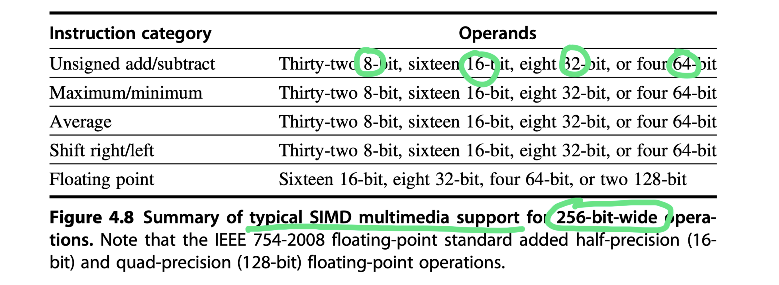
SIMD Instruction Set Extensions for Multimedia
- SIMD Multimedia Extension’s key idea
- many media applications operate on narrower data types
- Graphics systems would use 8 bits for colors and transparency
- Audio samples : 8 or 16 bits
- Partitioning the carry chains within, say, a 256-bit adder
- $\rightarrow$ Simultaneous operations on short vectors of
- Thirty-two 8-bit operands,
- Sixteen 16-bit operands,
- Eight 32-bit operands, or
- Four 64-bit operands
- $\rightarrow$ Simultaneous operations on short vectors of
- Small additional cost from partitioned adders
- many media applications operate on narrower data types
- Register file size?
- Vector architecture: Larger eg. 32 64-bit elements in each of 32 vector registers
- SIMD instructions: Fewer operands and thus use much smaller register files.
- SIMD extensions’s three major omissions in contrast to vector architecture
- No vector length registers
- So, need the addition of hundreds of instructions in MMX, SSE, AVX of x86
- No strided or gather/scatter data transfer instructions,
- Harder to vectorize programs
- No mask registers (changing recently)
- Harder to support conditional execution of elements
- $\rightarrow$ Harder for the compiler to generate SIMD code
- No vector length registers
- SIMD extensions in x86 architecture
- MMX in 1996: Repurposed the 64-bit floating point registers
- Eight 8-bit operations or four 16-bit operations simultaneously
- Joined by
- Parallel MAX and MIN operations
- A wide variety of masking and conditional instructions
- Ad hoc instructions that were believed to be useful in important media libraries
- Reused the floating-point data-transfer instructions to access memory
- Streaming SIMD Extensions (SSE) in 1999
- 16 separate 128-bit wide registers (XMM registers)
- Sixteen 8-bit operations, eight 16-bit operations, or four 32-bit operations
- Parallel single-precision floating-point arithmetic
- 16 separate 128-bit wide registers (XMM registers)
- SSE2 in 2001
- Added double-precision SIMD floating-point data types
- SSE3 in 2004
- SSE4 in 2007
- Four single-precision floating-point operations or
- Two parallel double-precision operations
- Ad hoc instructions
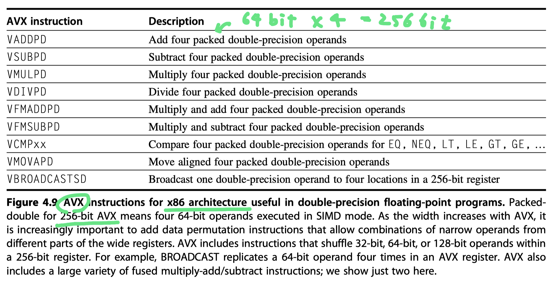
- Advanced Vector Extensions (AVX) in 2010
- Doubled the width of the registers again to 256 bits (YMM registers)
- Doubled #operations on all narrower data types.
- AVX2 in 2013
- Added 30 new instructions
- Gather (VGATHER) and vector shifts (VPSLL, VPSRL, VPSRA)
- AVX-512 in 2017
- Doubled the width again to 512 bits (ZMM registers)
- Doubled the number of the registers again to 32
- Added 250 new instructions
- Scatter (VPSCATTER) and mask registers (OPMASK)
- MMX in 1996: Repurposed the 64-bit floating point registers
- Programming model of SIMD extensions
- Accelerate carefully written libraries
- Recent 8x6 compilers are trying to generate such code
- Every time the width doubles, so must #SIMD instructions
- Why multimedia SIM extensions so popular?
- Cost little and easy to implement
- Less extra processor state $\rightarrow$ Better context switch times than vector architecture
- Require less memory bandwidth than vector architecture
- No page fault by a single instruction
- Vector architecture needs to deal with problems in virtual memory
- Easy to introduce instructions that can help with new media standards
- $\exists$ Concern about how well vector architectures can work with caches
-
- Once an architecture gets started on the SIMD path it’s very hard to get off it.
Programming Multimedia SIMD Architectures
-
Ad hoc nature of the SIMD extensions
- How to use these instructions?
- Through libraries
- Writing in assembly language
- Recently extensions
- More regular $\rightarrow$ More reasonable target for compliers
- Advanced compilers today
- Can generate SIMD floating-point instructions
- Programmers
- Align all the data in memory to the width of the SIMD unit
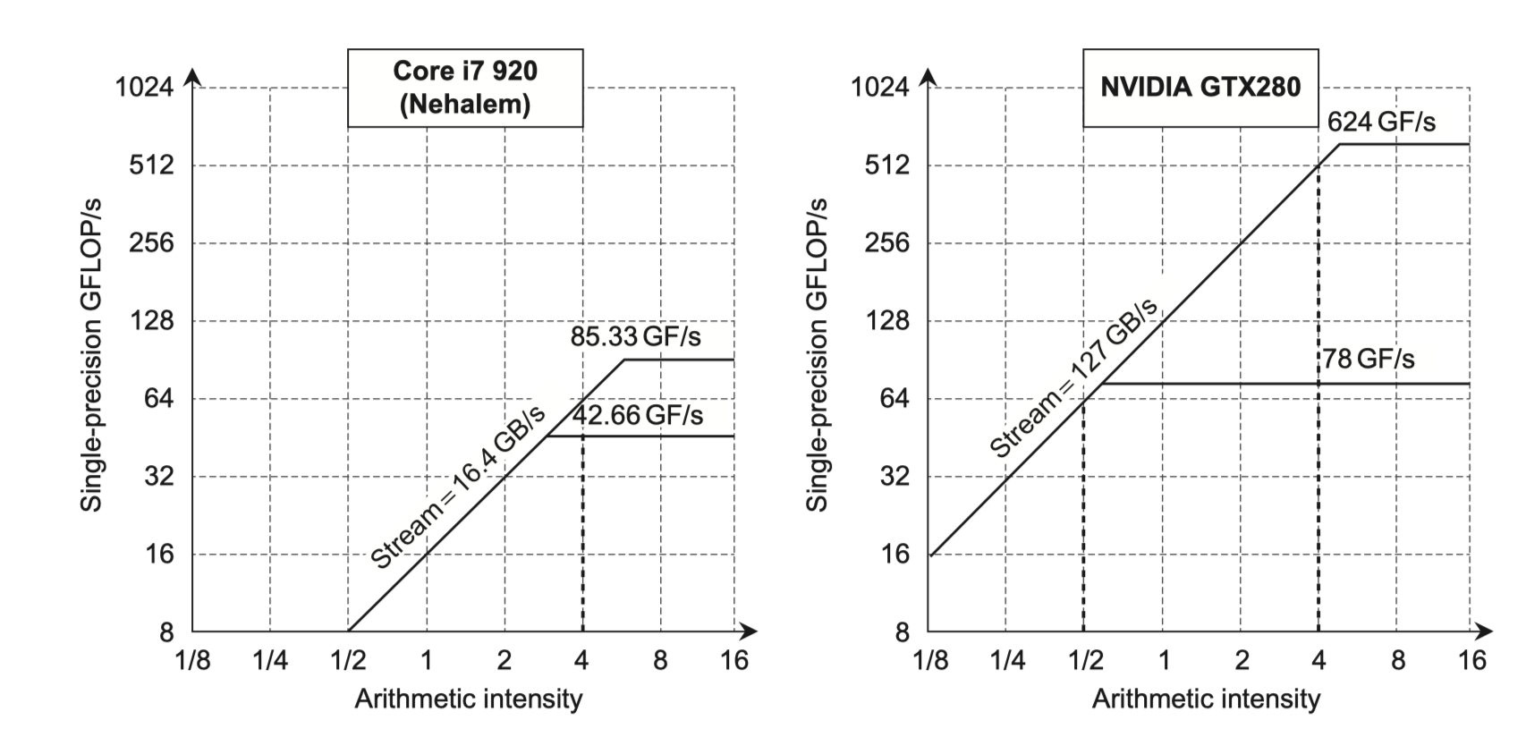
The Roofline Visual Performance Model
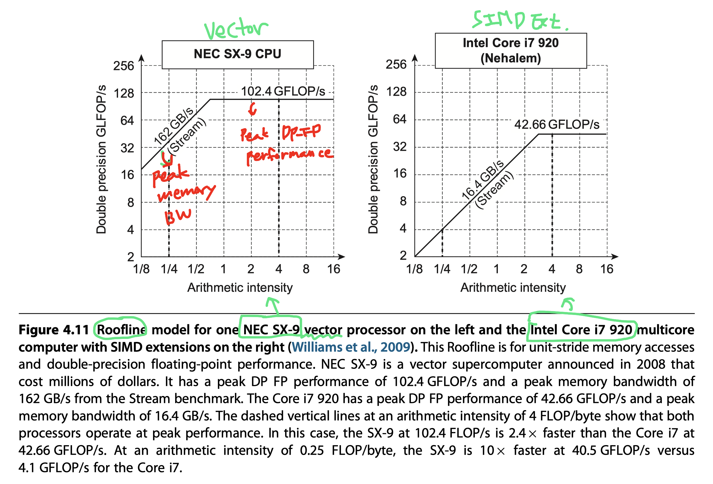
- Roofline
- One visual, intuitive way to compare potential floating-point performance of variations of SIMD architectures
- Upper bound on performance of a kernel depending on its arithmetic intensity
- Ties together in a two-dimensional graph
- Floating-point performance
- Memory performance
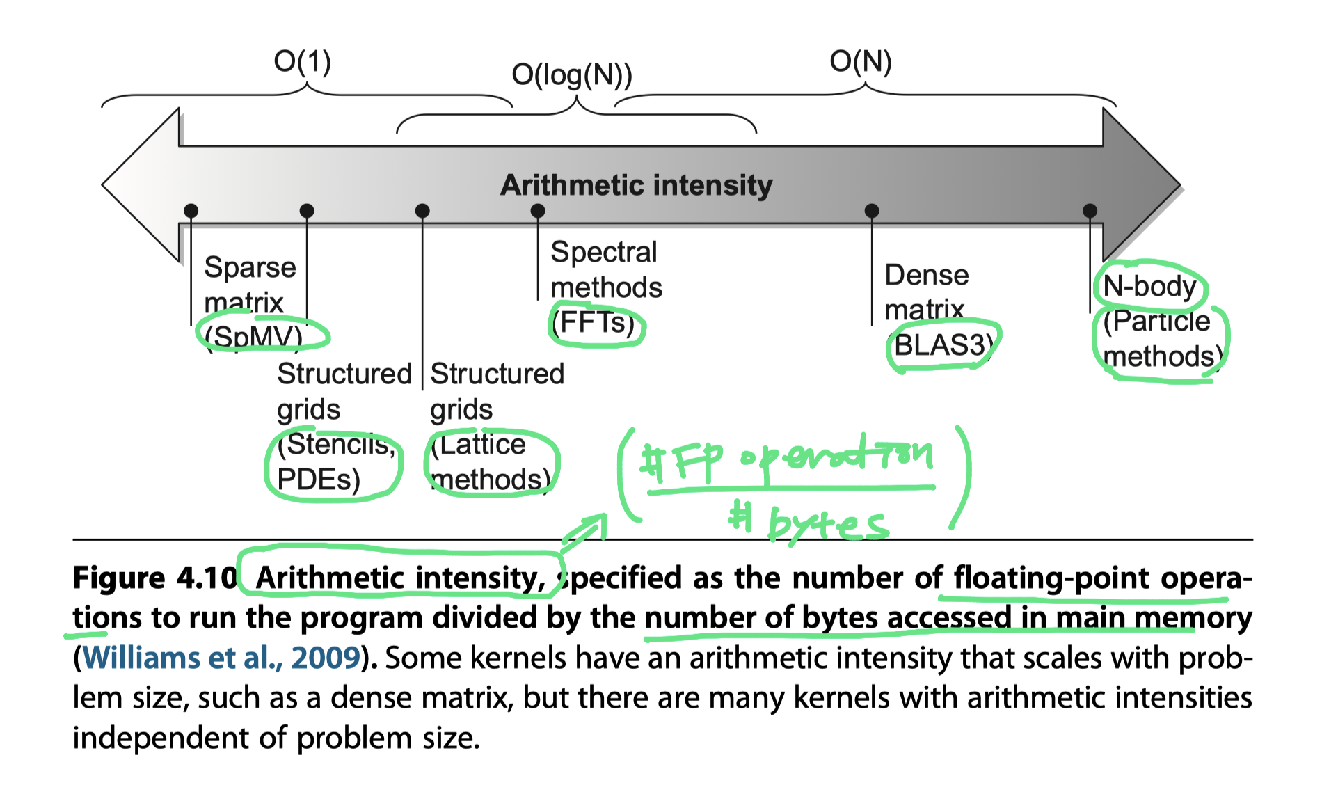
- Arithmetic intensity
- Arithmetic intensity
- The ratio of floating-point operations per byte of memory accessed
- #FP-operations/#bytes transferred to main memory

Graphics Processing Units
-
The primary ancestors of GPUs = “Graphics accelerators”
- GPU designer’s question
- Given the hardware invested to do graphics well,
- “How can we supplement it to improve the performance of a wider range of applications?”
- Traditional role of graphics acceleration?
- See “Graphics and Computing GPUs,” by John Nickolls and David Kirk (Appendix A in the 5th edition)
Programing the GPU
- Challenges for the GPU programmer
- Good performance on the GPU
- Coordinating
- Scheduling of computation on the system processor and the GPU
- Transfer of data between system memory and GPU memory.
- Every type of parallelism in GPUs
- Multithreading
- MIMD
- SIMD
- Instruction level
- CUDA
- Compute Unified Device Architecture
- NVIDIA’s C-like language and programming environment
- Produces
- C/C++ for system processor (host)
- C/C++ dialect for the GPU (device)
- Similar to OpenCL
- Levels of parallelism
- CUDA Thread:
- The lowest level of parallelism + programming primitive
- So, SIMT (Single instruction, multiple thread)
- Thread Block
- Threads are blocked and executed in groups of thread
- Multithreaded SIMD Processor = Hardware that executes a whole block of threads
- Grid
- Code that runs on a GPU that consists of a set of Thread Blocks
- CUDA Thread:
- CUDA program details
-
__device__ or __global__: GPU- CUDA variables declared with
__device__are allocated to GPU memory, which is accessible by all multithreaded SIMD Processors.
- CUDA variables declared with
-
__host__: System processor - Extended function call syntx
name < <<dimGrid, dimBlock>> > (...parameter list...)
-
dimGrid: Code dimension in Thread Blocks-
blockIdx: Identifier for blocks
-
-
dimBlock: Code dimension in threads-
threadIdx: Identifier for each thread in a block
-
-
- C code for DAXPY loop
- DAXPY :
y <- y + axwith DFP scalar a, vector x, vector y - n : Vector dimension
- DAXPY :
1
2
3
4
5
6
7
8

// Invoke DAXPY
daxpy(n, 2.0, x, y);

// DAXPY in C
void daxpy(int n, double a, double *x, double *y) {
	for (int i = 0; i < n; ++i)
		y[i] = a*x[i] + y[i];
}
- CUDA code for DAXPY loop
- $n$ threads, one per vector element
- 256 CUDA Threads per Thread Block in a multithreaded SIMD Processor
- GPU functions starts by calculating the corresponding element index i based on
- The block ID,
- The number of threads per block, and
- The thread ID.
- Vector compilers rely on a lack of dependence between iteration of a loop (loop-carried dependences)
- Explicitly determine the parallelism in CUDA
- Grid dimensions
- #Threads per SIMD Processors
- Assign a single thread to each element
- No need to synchronize between threads when writing results to memory
1
2
3
4
5
6
7
8
9
10
11

// Invoke DAXPY with 256 threads per Thread Block
__host__
int nblocks = (n + 255) / 256;
daxpy<<<nblocks, 256>>>(n, 2.0, x, y);

// DAXPY in CUDA
__global__
void daxpy(int n, double a, double *x, double *y) {
	int i = blockIdx.x*blockDim.x + threadIdx.x;
	if (i < n) y[i] = a*x[i] + y[i];
}
- Hardware handles parallel execution and thread management
- Thread Blocks execute independently
- Different Thread Blocks cannot communicate directly
- Although they can coordinate using atomic memory operations in global memory
- Programmers must
- Think in terms in of SIMD operations
- Keep the GPU hardware in mind
- $\rightarrow$ It could hurt programmer productivity
- In detail,
- Keep groups of 32 threads together in control flow,
- Create many more threads per multithreaded SIMD Processors to hide latency to DRAM
- Keep the data addresses localized in one or a few blocks of memory to get the expected memory performance
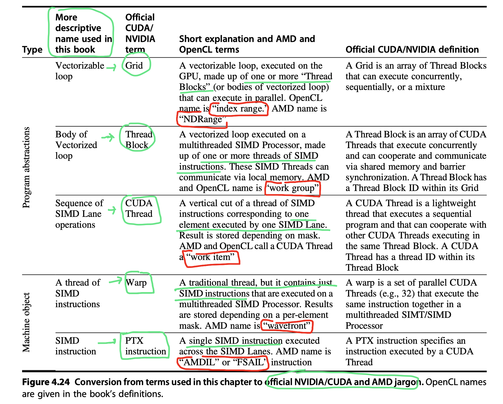
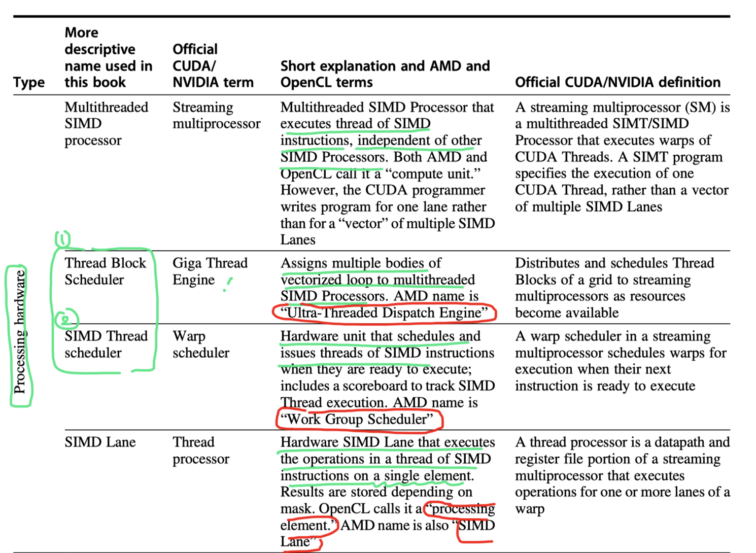
NVIDIA GPU Computational Structures
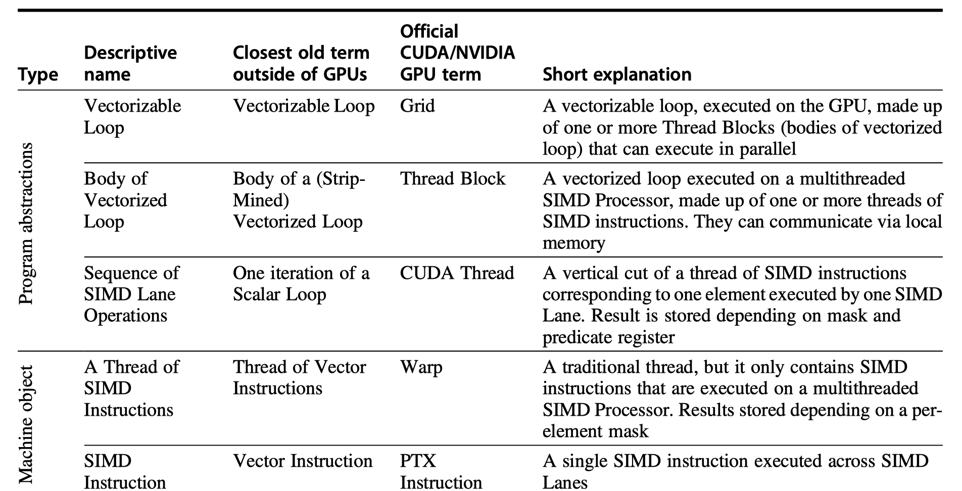
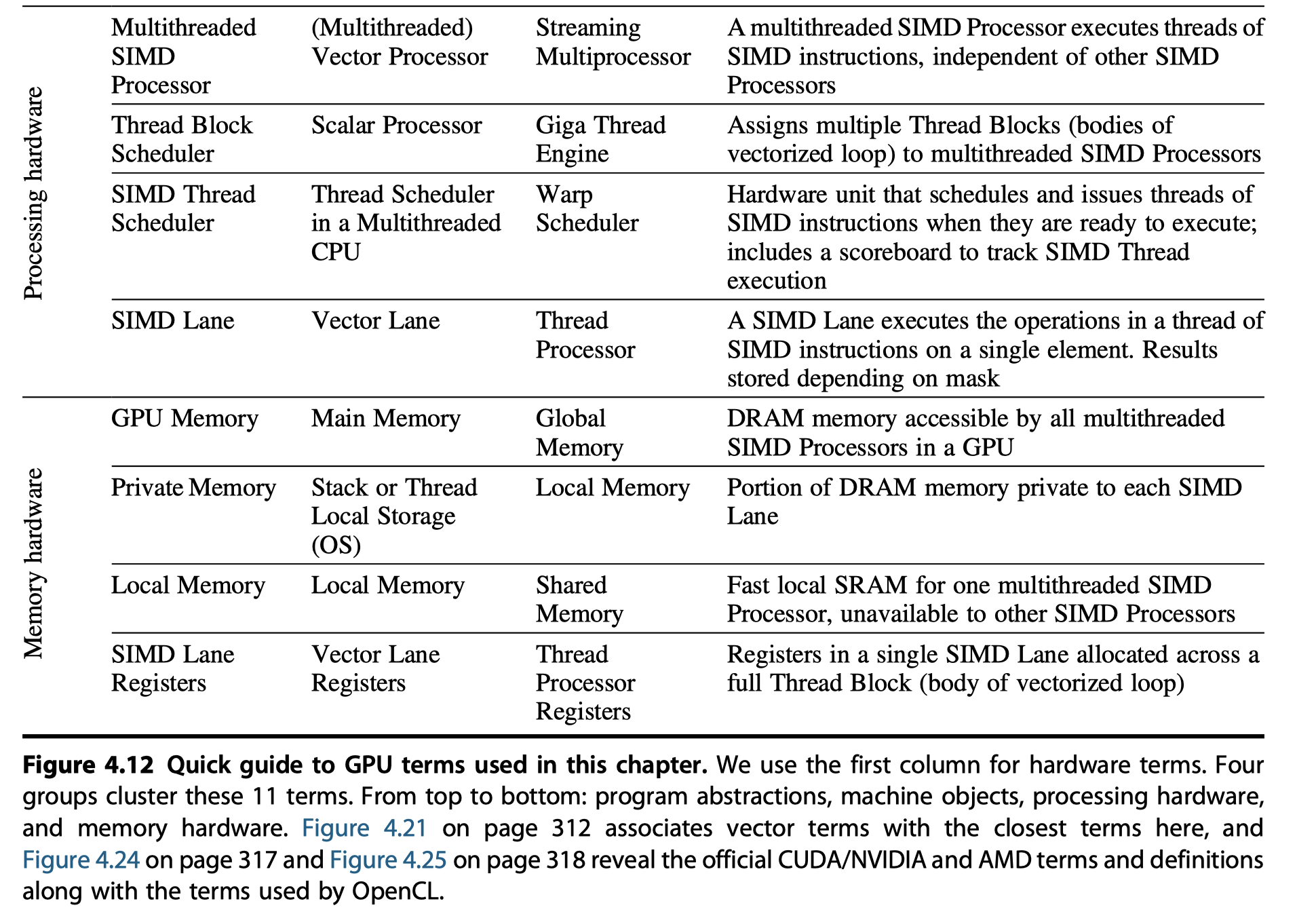
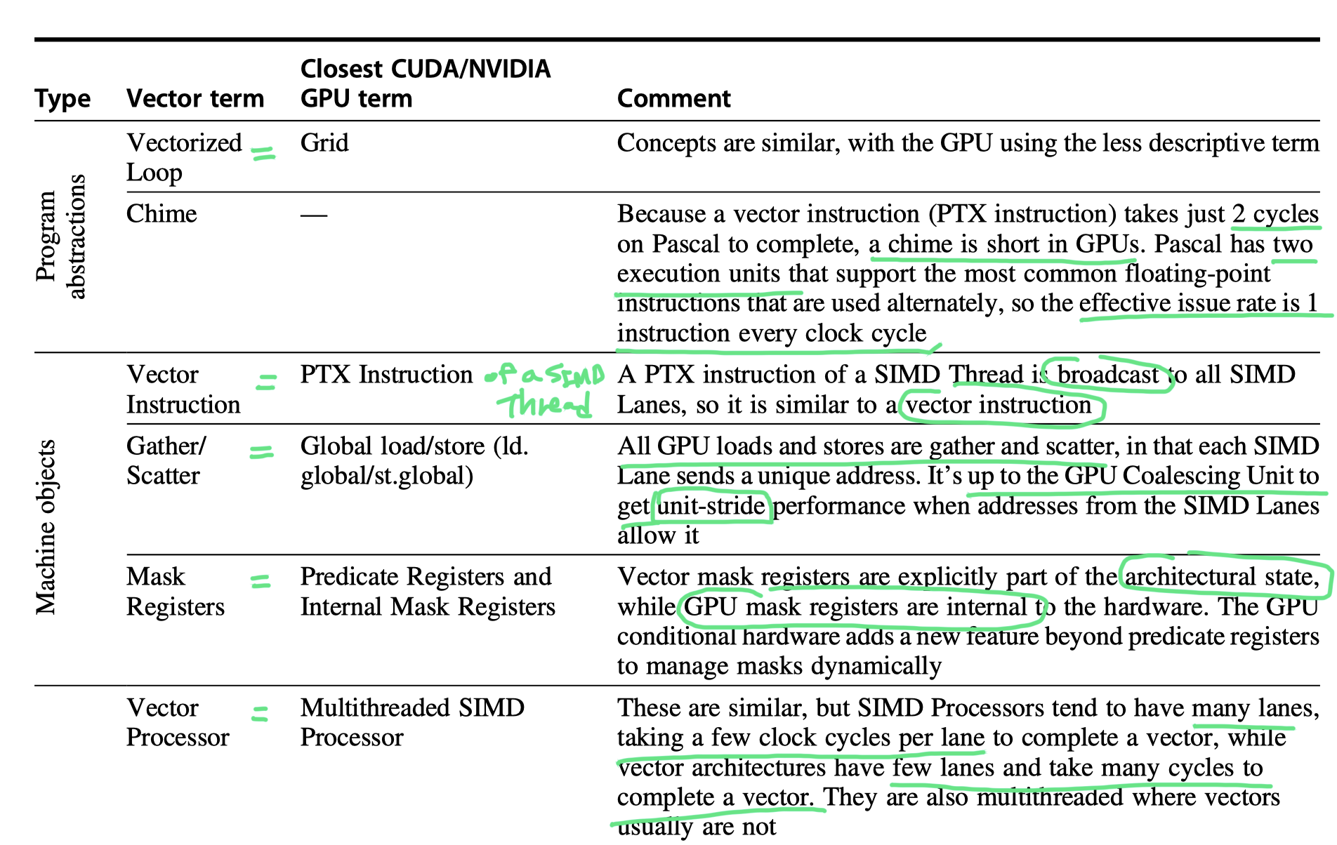
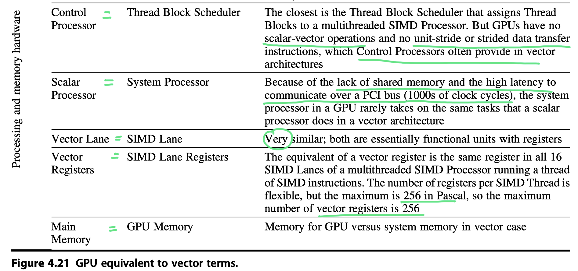
- Renaming the official jargon of NVIDIA GPUs
- Similarity to vector architectures
- GPUs work well only with data-level parallel problems
- Gather-scatter data transfers
- Mask registers
- Even more registers than do vector processors
- Both requires programmers to think in groups of SIMD operations
- Difference to vector architectures
- Software-features in vector architecture $\rightarrow$ Hardware implementation in GPUs (due to lack of scalar processor)
- GPU also rely on multithreading within a single multithreaded SIMD processors to hide memory latency
- Grid
- Code that runs on a GPU that consists of a set of Thread Blocks.
- A grid ~ a vectorized loop
- A Thread Block ~ body of that loop after it has been strip-mined (i.e. Strip-mined vector loop)
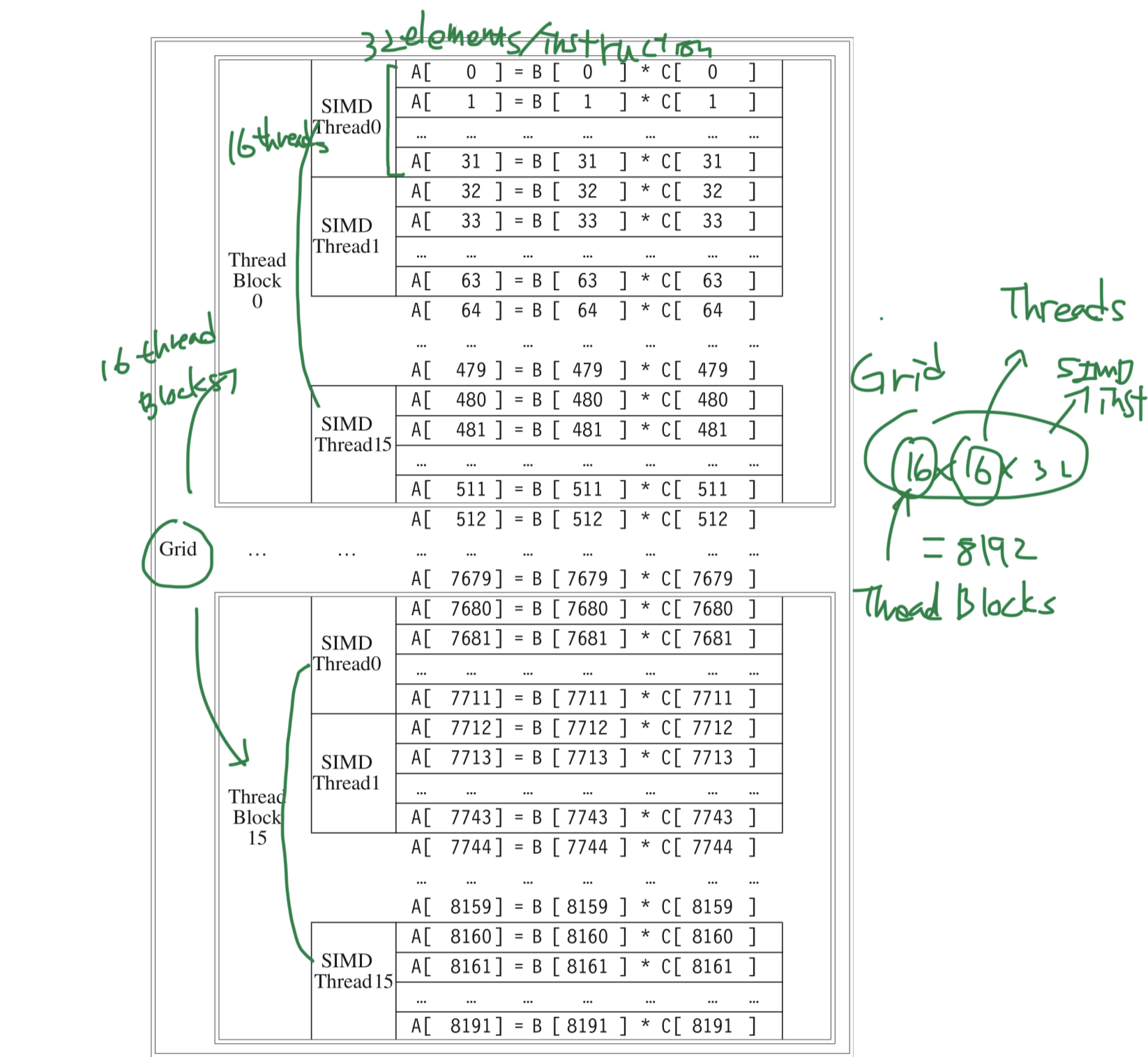
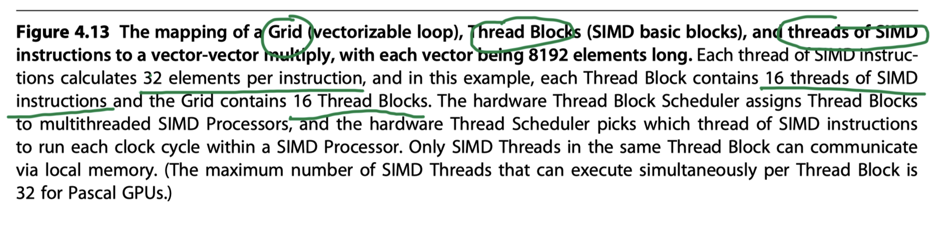
- Vectorization example with CUDA
- Multiply two vectors with n = 8192
- Code for the whole 8192 elements = Grid = Vectorized loop
- Grid
- 16 Thread Blocks with up to 512 elements = Body of a vectorized loop
- 16 Thread Blocks = $8192\div 512$
- Thread Block
- 512 elements (CUDA Threads) in a Thread Block
- = 16 SIMD Threads in a Thread Block
- Assigned to a multithreaded SIMD Processor
- By the Thread Block Scheduler
- Implemented in hardware
- SIMD Thread
- 1 SIMD Thread = 1 SIMD instruction = 32 element wide = 32 CUDA Threads
- SIMD Lanes
- 16 SIMD Lanes
- 32/16 = 2 cycles to complete a SIMD instruction
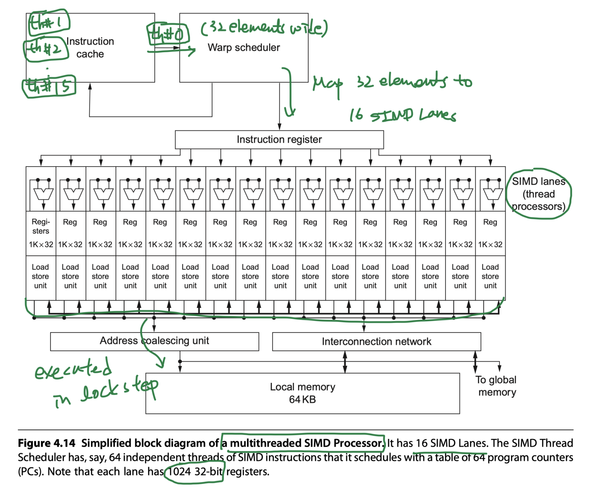
- Mapping to GPU hardware
- A Multiprocessor composed of multithreaded SIMD Processors
- Each multithreaded SIMD Processor
- Full processor with separate PCs and are programmed using threads
- Many parallel functional units instead of a few that are deeply pipelined, as in a vector processor
- Thread of SIMD instructions
- Basic machine object
- Each thread has its own PC (Not PC per element)
- Executed in lock step
- Scheduled only at the beginning
- Run on a multithreaded SIMD Processor
- eg. 32 wide SIMD instruction executed by 16 SIMD Lanes
- Parallel functional units = SIMD Lanes
- Quite similar to vector lanes in vector architecture
- Two levels of hardware schedulers:
- (1) Thread Block Scheduler
- Provide transparent scalability across GPU models with different # multithreaded SIMD Processors
- Assigns Thread Blocks (Bodies of a vectorized loop) to multithreaded SIMD Processors
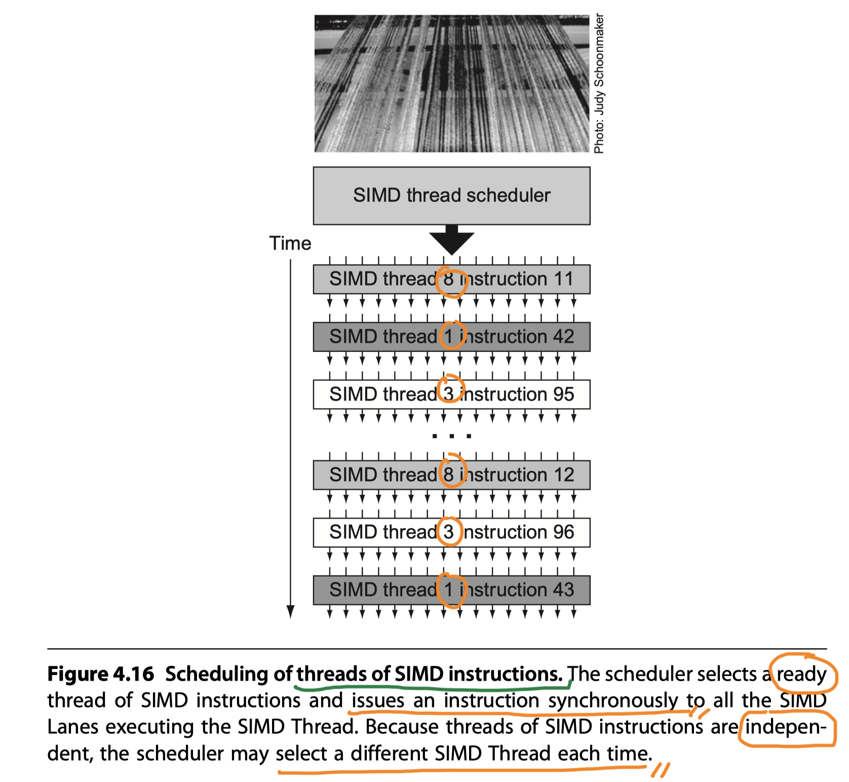
- (2) SIMD Thread Scheduler
- Within a SIMD Processor
- Knows which threads of SIMD instructions are ready
- Sends them off to a dispatch unit to be executed
- Includes a scoreboard to keep track of up to 64 threads of SIMD instructions to see which SIMD instruction is ready to go
- eg. Variable latency of memory instructions due to TLB or cache miss
- Picks threads of SIMD instructions in different order over time (Figure 4.16)
- (1) Thread Block Scheduler
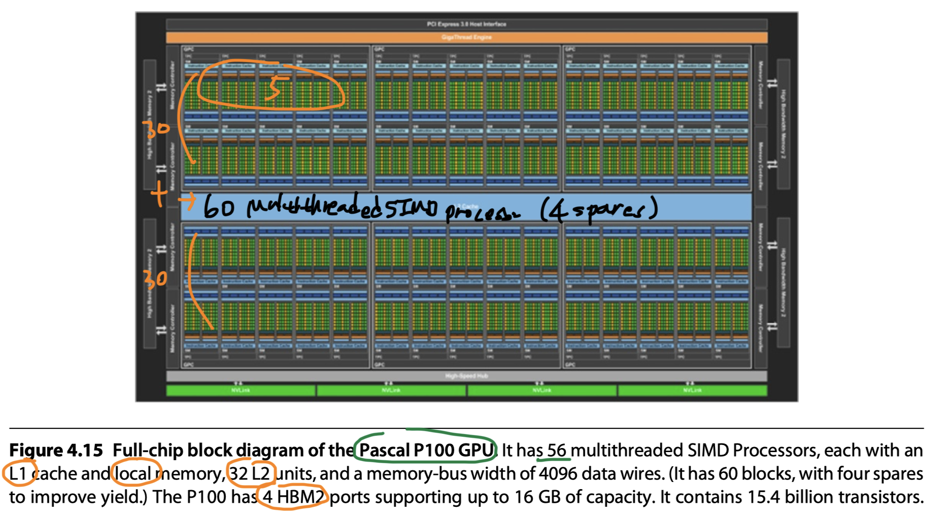
- e.g. Pascal P100:
- 56 multithreaded SIMD Processors in P100
- 16 physical SIMD Lanes
- Map 32-wide thread of SIMD instructions
- So, 2 cycles to complete a SIMD instruction
- Wide but shallow
- Mapping to vector processor
- #Lanes = 16
- Vector length = 32
- Chime = 2 clock cycles
- Registers
- A SIMD Processor has 32K ~ 64K 32-bit registers
- 1024 per lane in Figure 4.14
- Divided logically across the SIMD lanes
- Each SIMD Thread is limited to no more than 256 registers
- Trade-off between register use and maximum number of threads!
- (#Register/Thread) $\times$ #Threads) = 32K~64K
- Example
- Thread block A = 16 SIMD Threads $\times$ 36 Registers/Thread
- Thread block B = 32 SIMD Threads $\times$ 20 Registers/Thread
- So, Dynamically allocate physical registers on demand to different threads in any order
- Variability $\rightarrow$ Fragmentation, Unavailable register
- Hardware records the location of each Thread Block’s register in the register file
- It can be anywhere, so …
- Need routing, arbitration, banking in the hardware
- CUDA Thread
- Just a vertical cut of a thread of SIMD instructions
- Corresponding to one element executed by one SIMD Lane
NVIDIA GPU Instruction Set Architecture
- PTX (Parallel Thread Execution) instruction set architecture
- Low-level parallel thread execution virtual machine and instruction set architecture used in Nvidia’s CUDA programming environment
- (Step 1) The NVCC compiler translates code written in CUDA, a C++-like language, into PTX instructions (an assembly language represented as ASCII text),
- (Step 2) The graphics driver contains a compiler which translates the PTX instructions into the executable binary code which can be run on the processing cores of Nvidia GPUs.
- Abstraction of the hardware instruction set
- The hardware instruction set is hidden from the programmer
- Provide a stable instruction set for compilers
- Describe the operations on a single GUDA Thread
- Map one-to-one with hardware instructions
- One PTX instruction can expand to many machine instructions and vice versa
- Uses an unlimited number of write-once registers
- The compiler must run a register allocation procedure to map the PTX registers to a fixed number of read-write hardware registers available on the actual device
- Optimizer
- Runs subsequently and can reduce register use even further
- Eliminates dead code
- Fold instructions together
- Calculates
- Places where branches might diverge
- Places where diverged paths could converge.
- PTX vs x86
- Both translate to an internal form (microinstructions for x86, hardware instruction for PTX)
- Translation happens in
- Hardware & Runtime on x86
- Software & Load-time on PTX
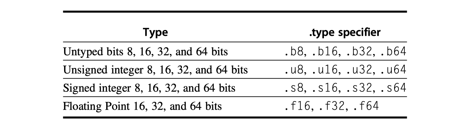
- PTX format
-
opcode.type d, a, b, c- d: Destination operand
- a, b, c: Source operands
-
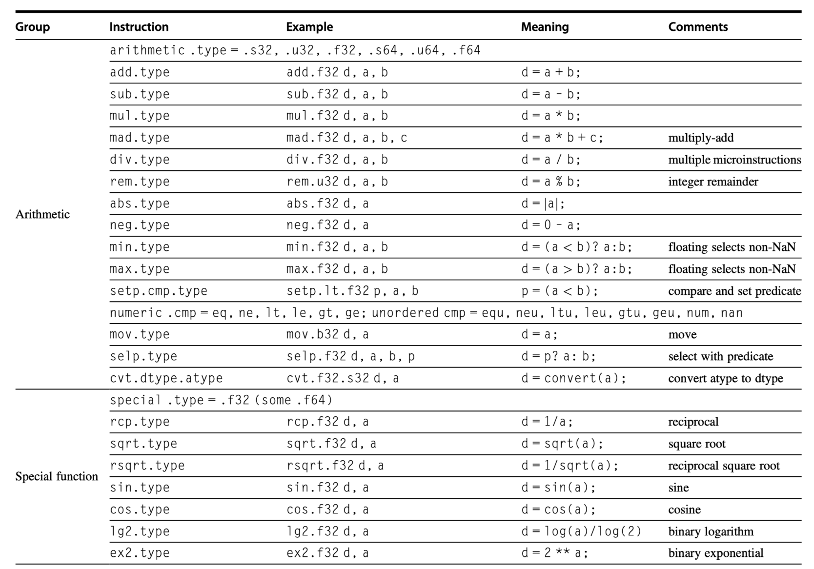
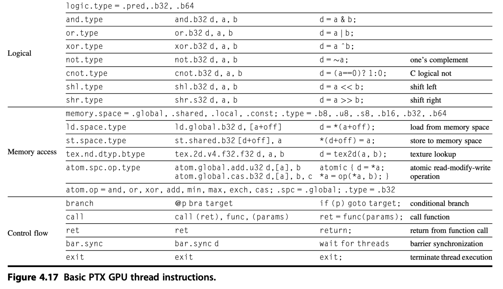
- PTX instruction set
- Predicated by 1-bit predicate registers (Set by
setp: Set predicate instruction)- Gives conditional branches
- Control flow instructions:
- Functions:
call,return - Thread:
exit,branch - Barrier synchronization for threads within a Thread Block:
bar.sync
- Functions:
- Predicated by 1-bit predicate registers (Set by
- Virtual registers
-
R0,R1, … are for 32-bit values -
RD0,RD1, … are for 64-bit registers - Assignment of virtual registers to physical registers at load time with PTX
-
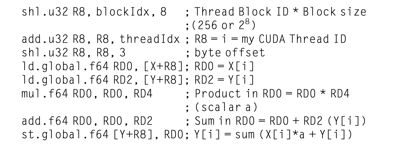
- Sequence of PTX instructions for one iteration of DAXPY loop
- One CUDA Thread $\rightarrow$ (
blockIdx,threadIdx) - The first three PTXs
- Calculate unique element byte
- Following PTXs
- Load two operands
- Multiply, Add, Store
- No separate instructions for
- Sequential data transfers,
- Strided data transfers, and
- Gather-scatter data transfers.
- All data transfers are gather-scatter!!!!
- One CUDA Thread $\rightarrow$ (
- Special Address Coalescing hardware
- Efficient sequential data transfer
- When?
- SIMD Lanes within a thread of SIMD instructions are collectively issuing sequential address
- Notifies the Memory Interface Unit to request a block transfer of 32 sequential words
- Programmer must ensure that adjacent CUDA Threads access nearby addresses at the same time
Conditional Branching in GPUs
- Strong similarities between how vector architectures and GPUs handle IF statements
- Explicit predicate registers
- Difference?
- Vector architectures: implementing the mechanism largely in software with limited hardware support
- GPUs: making use of even more hardware
- Manage when a branch diverges into multiple execution paths and when the paths converge
- GPU branch hardware uses internal masks
- A branch synchronization stack
- Instruction markers
- Control flow of one CUDA Thread described by PTX instructions
- Functions:
call,return - Thread:
exit,branch - Barrier synchronization for threads within a Thread Block:
bar.sync - Individual per-thread-lane predication of each instruction
- Specified by the programmer with per-thread-lane 1-bit predicate registers
- Functions:
- PTX assembler (PTX $\rightarrow$ Hardware instructions)
- Analyzes the PTX branch graph
- Optimizes it to the fastest GPU hardware instruction sequence
- A simple outer-level IF-THEN-ELSE statement ?
- Solely predicated GPU instructions without any GPU branch instructions
- More complex one: Branch divergence
- Mixture of predication and
- GPU branch instructions with special instructions and markers that
- Use the branch synchronization stack
- To push a stack entry when some lanes branch to the target address, while others fall through
- This mixture is also used
- When a SIMD Lane executes a synchronization marker or converges,
- Which pops a stack entry and branches to the stack-entry address with the stack-entry thread active mask
- Identifies loop branches?
- Generates GPU branch instructions that
- Branch to the top of the loop,
- Along with special stack instructions
- To handle individual lanes
- Breaking out of the loop and
- Converging the SIMD Lanes when all lanes have completed the loop.
- GPU indexed jump and indexed call instructions push entries on the stack so that
- When all lanes complete the switch statement or function call, the SIMD Thread converges.
- A simple outer-level IF-THEN-ELSE statement ?
- Control flow of one CUDA Thread described by GPU hardware instruction level
-
branch,jump,jump indexed,call,call indexed,return,exit, - Special instructions that manage the branch synchronization stack
-
- Stack in GPU
- $\exists$ Stack for each SIMD Thread
- A stack entry $\ni$ Identifier token, a target instruction address, and a target thread-active mask
- Special instructions that push stack entries for a SIMD Thread
- Special instructions and instruction markers that pop a stack entry or unwind the stack to a specified entry and branch to the target instruction address with the target thread-active mask
- A GPU set predicate instruction
setp- Evaluates the conditional part of the IF statement
- PTX branch instruction then depends on that predicate.
- If the PTX assembler generates predicated instructions with no GPU branch instructions,
- It uses a per-lane predicate register to
- Enable or
- Disable each SIMD Lane for each instruction
- It uses a per-lane predicate register to
- The SIMD instructions in the threads inside the THEN part of the IF statement broadcast operations to all the SIMD Lanes.
- Lanes with the predicate set to 1 perform the operation and store the result,
- Lanes with the predicate set to 1 don’t perform an operation or store a result
- For the ELSE statement,
- The instructions use the complement of the predicate (relative to the THEN statement),
- So the SIMD Lanes that were idle now perform the operation and store the result
- while their formerly active siblings don’t.
- At the end of the ELSE statement,
- the instructions are unpredicated
- If the PTX assembler generates predicated instructions with no GPU branch instructions,
- Nested IF statement?
- A mix of predicated instructions and GPU branch and special synchronization instructions for complex control flow
- Doubly nested IF statements with equal-length paths run at 25% efficiency
- Triply nested at 12.5% efficiency, and so on.
- PTX assembler sets a “branch synchronization” marker
- On appropriate conditional branch instructions
- That pushes the current active mask
- On a stack inside each SIMD Thread
- If the conditional branch diverges
- i.e. Some lanes take the branch but some fall through
- It
- Pushes a stack entry and
- Sets the current internal active mask based on the condition
- A branch synchronization marker
- Pops the diverged branch entry and
- Flips the mask bits before the ELSE portion.
- At the end of the IF statement,
- The PTX assembler adds another branch synchronization marker
- That pops the prior active mask off the stack into the current active mask.
- If all the mask bits are set to 1,
- Then the branch instruction at the end of the THEN
- Skips over the instructions in the ELSE part.
- Then the branch instruction at the end of the THEN
- There is a similar optimization for the THEN part in case all the mask bits are 0
- Because the conditional branch jumps over the THEN instructions.
- Parallel IF statements and PTX branches often use branch conditions that are unanimous (all lanes agree to follow the same path)
- such that the SIMD Thread does not diverge into a different individual lane control flow.
- The PTX assembler optimizes such branches to skip over blocks of instructions that are not executed by any lane of a SIMD Thread.
- This optimization is useful in conditional error checking, for example, where the test must be made but is rarely taken.
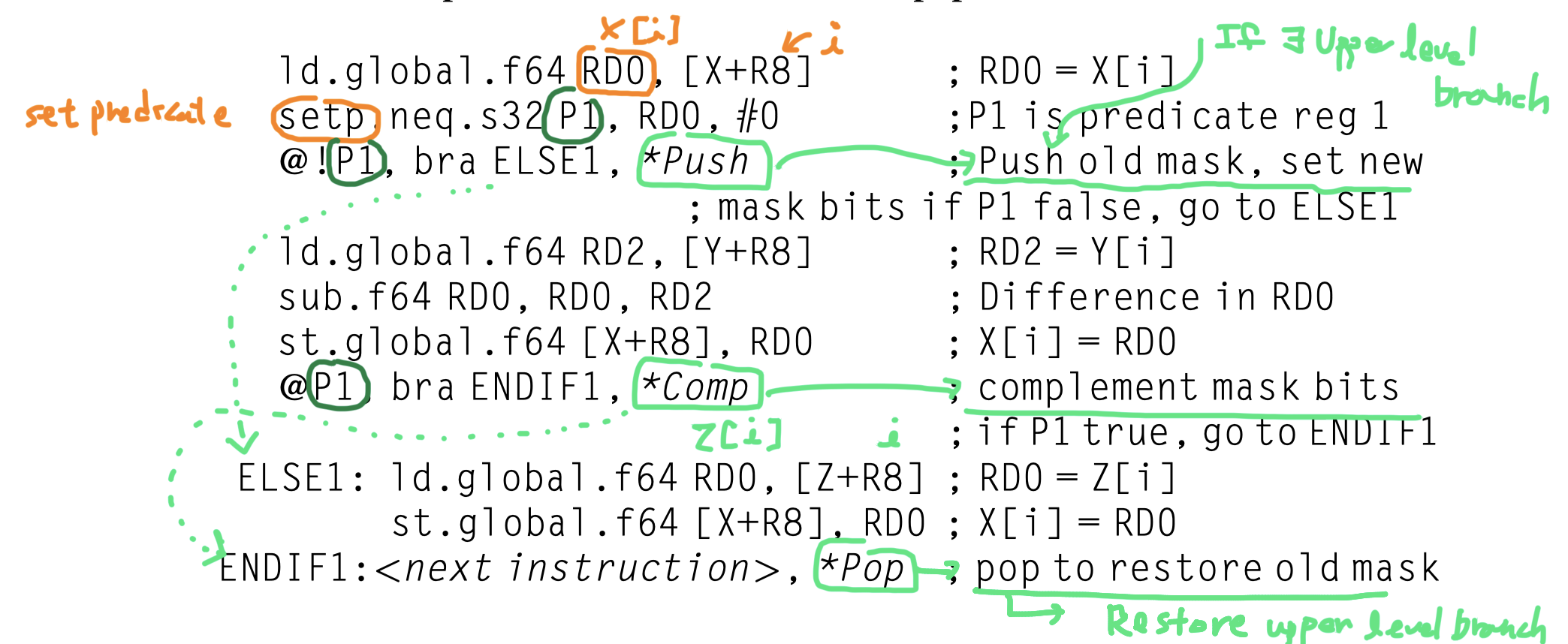
- Code with a conditional statement
1
2
3

if (X[i] != 0)
  X[i] = X[i] – Y[i];
else X[i] = Z[i];
- Converted to PTX instructions
- R8 = Scaled thread ID
- Branch synchronization markers inserted by the PTX assembler
-
*Push: Push the old mask -
*Comp: Complement the current mask -
*Pop: Pop to restore the old mask
-
- This flexibility makes it appear (i.e. gives illusion) that an element has its own program counter;
- Actually it’s not (One PC per thread, not per element)
- Helpful in the early stages of program development with poor performance
- Gives illusion that each CUDA Thread (= each element in a thread of SIMD instructions) acts independently!!
- That’s why it is called as CUDA “Thread”, although it is not really a thread that must be independent to other thread
- So, NVIDIA says that CUDA “Threads” executed in lock step, which means that CUDA Thread are just elements in a thread of SIMD instructions
- Do CUDA threads execute in lockstep for O(n) operations? from StackOverfLow
- Conditional execution is done in
- Runtime by hardware in GPUs
- Compile time by compiler in vector processors
- Vector compilers do
- Double IF-conversion
- generating four different masks.
- Execution is the same with GPUs
- More overhead instructions executed for vectors
- Possible to use scalar processor if only small portion of the mask bits are 1s.
- Vector compilers do
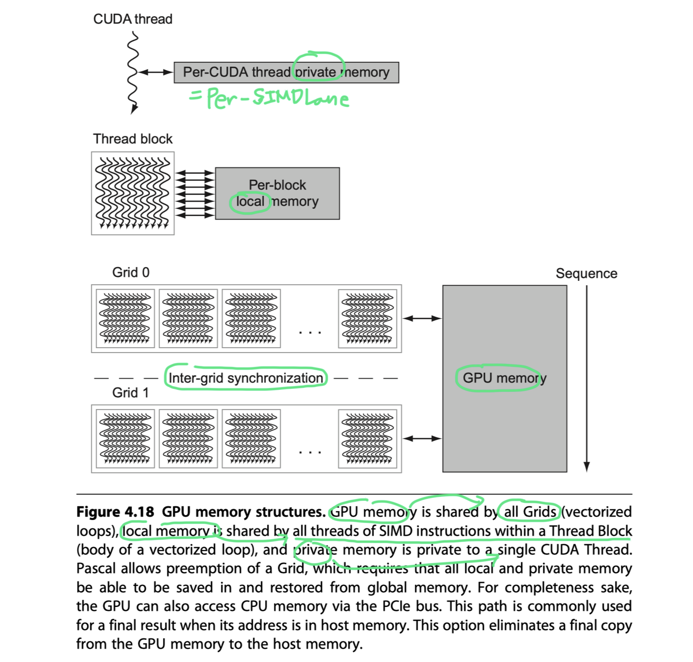
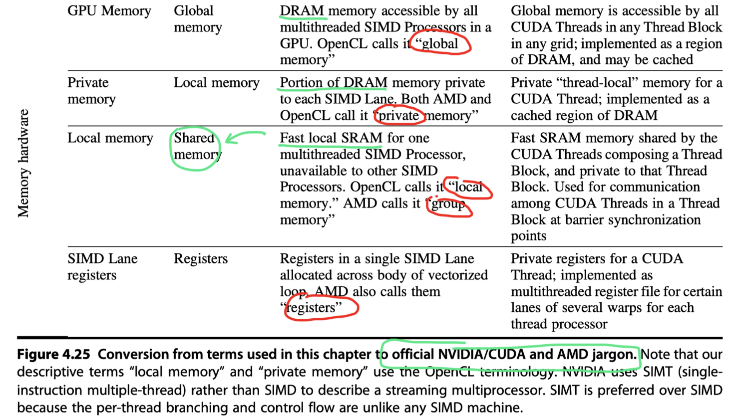
NVIDIA GPU Memory Structures
- Private memory
- A private section of off-chip DRAM
- Allocated to each SIMD Lane (= each CUDA thread) in a multithreaded SIMD Processor
- Used for
- Stack frame
- Spilling registers
- Private variables that don’t fit in the registers
- SIMD Lanes do not share private memories
- GPU caches
- Private memories in the L1 and L2 caches
- To aid register spilling and to speed up function calls
- Unavailable to the system processor (host)
- Local memory
- On-chip memory that is local to each multithreaded SIMD Processor
- A small scratchpad memory with
- Low latency ( A few dozen clocks )
- High bandwidth ( 128 bytes/clock )
- Limited in size ~ 48 KiB
- Programmer can store data that needs to be reused, either by
- The same thread or
- Another thread in the same Thread Block
- Shared by the SIMD Lanes within a multithreaded SIMD Processor
- Not shared between multithreaded SIMD Processors
- Dynamically Allocated to a Thread Block
- By Multithreaded SIMD Processor
- Freed when all the threads of the Thread Block exit
- Private to that Thread Block
- Carries no state between Thread Blocks executed on the same processor
- Unavailable to the system processor (host)
- GPU memory
- Off-chip DRAM shared by the whole GPU and all Thread Blocks
- Accessed by the system processor (host)
- Streaming caches
- Not rely on large caches
- The chip area used for large L2 and L3 caches in system processors is spent instead on computing resources and on the large number of registers to hold the state of many threads of SIMD instructions
- Hide long latency to DRAM by relying on extensive multithreading of threads of SIMD instructions
- In contrast, vector load/stores amortize the latency across many elements by paying the latency only once and then pipeline the rest of the accesses
- So, similar philosophy
- Little’s Law from queuing theory
- Q: If hiding latency behind many thread is so good, why do we still need caches?
- A: Many threads for low latency require many registers, that are expensive
- So, cache is still good to lower latency and thereby mask potential shortages of the number of registers
- Not rely on large caches
- To improve memory bandwidth and reduce overhead
- Address Coalescing
- PTX data transfer instructions
- In cooperation with the memory controller
- Coalesce individual parallel thread requests
- From the same SIMD Thread together
- Into a single memory block request,
- When the addresses fall in the same block
- PTX data transfer instructions
- GPU memory controller will also
- Hold requests and
- Send ones together
- To the same open page
- Address Coalescing
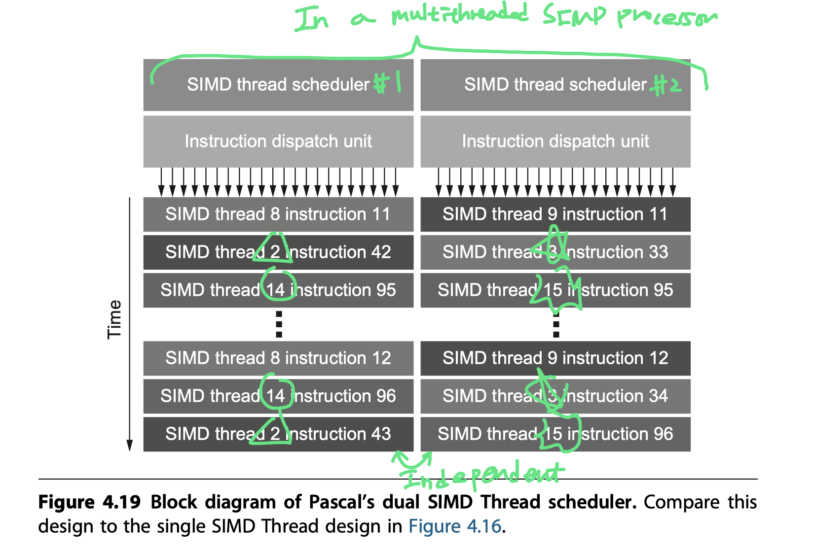
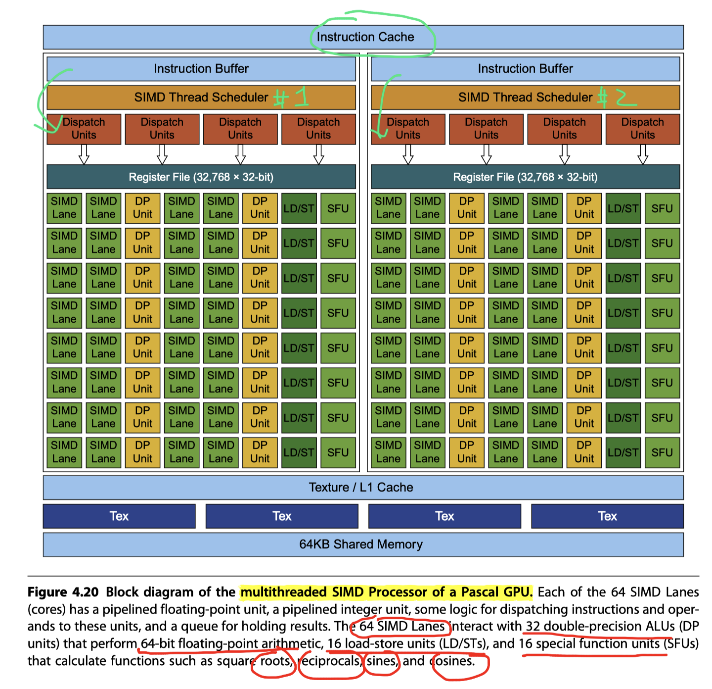
Innovations in the Pascal GPU Architecture
- Pascal architecture
- Introduced in April 2016
- GeForce GTX1060~1080
- To increase hardware utilization
- Two SIMD Thread Schedulers per SIMD Processor
- Each with multiple instruction dispatch units
- $\rightarrow$ Selects two threads of SIMD instructions
- Issues one instruction
- From each
- To two sets of
- 16 SIMD Lanes,
- 16 load/store units,
- Or 8 special function units
- Two threads of SIMD instructions are scheduled each clock cycle
- Allowing 64 lanes to be active
- No dependence between the two threads
- No need to check
- Analogous to
- A multithreaded vector processor that
- Can issue vector instructions from two independent threads
- Four main innovations of Pascal
- Fast single-precision, double-precision, and half-precision floating-point arithmetic
- Atomic memory operations $\ni$ FP-add for HFP, SFP, DFP
- High-bandwidth memory
- Stacked HBM2 with 4096 data wires \@ 0.7 GHz & 732 GB/s
- High-speed chip-to-chip interconnect
- NVLink communication between GPUs up to 20GB/s in each direction
- 4 NVLink in a GPU
- Aggregate chip-to-chip BW = 160 GB/s per chip
- 2, 4, 8 GPUs
- Possible to be connected to CPU (IBM Poewr9 CPU)
- Coherent view of memory between all GPUs and CPUs
- Provides also cache-to-cache communication
- Unified virtual memory and paging support
- Page-fault capabilities within a unified virtual address space
- Single virtual address across all the GPUs and CPUs in a single system
- When a thread accesses an address that is remote
- A page of memory is transferred to the local GPU for subsequent use
- Simplifies the programming model by providing demand paging instead of explicit memory copying between CPU and GPU or between GPUs
- Need to care to avoid excessive page movement
- Fast single-precision, double-precision, and half-precision floating-point arithmetic
Similarities and Differences Between Vector Architectures and GPUs
-
A SIMD processor ~ a vector processor
- Multiple SIMD Processor act as independent MIMD cores
- ~ Many vector computer
- Tesla P100
- 56-core machine with hardware support for multithreading
- Each core has 64 lanes
- Difference to vector processor = Multi-threading!
- Missing from vector processors
- Registers
- RV64V:
- Register file holds entire vectors - that is, a contiguous block of elements
- 32 vector registers with perhaps 32 elements = 1024 elements
- GPU:
- A single vector in a GPU will be distributed across the registers of all SIMD Lanes
- A GPU thread of SIMD instructions = Up to 256 registers with 32 elements each = 8192 elements
- These extra registers supports multithreading
- RV64V:
- Lanes
- Vector: 2~8 lanes $\rightarrow$ 4 to 16 cycle chime for vector length 32
- GPU: 8~16 lanes $\rightarrow$ 2 or 4 cycle short chime for 32 element SIMD Thread
- Closer to SIMD design than vector processor design
- All memory instruction in GPU = Gather for load, scatter for store
- The explicit unit-stride load and store instructions of vector architectures
- vs the implicit unit stride of GPU programming
- Reason why writing efficient GPU code requires that programmers think in terms of SIMD operations, even though the CUDA programming model looks like MIMD
- Memory latency hiding
- Vector architectures
- Amortize across all the elements of vector by having deeply pipelined access
- Pay the latency only once
- Vector load/store = Block transfer between memory and vector registers
- GPUs
- Hide latency using multithreading
- Continuous memory access $\rightarrow$ The first thread pay the latency once
- Recent Idea
- Add multithreading to vector architecture!
- Vector architectures
- Conditional branch instruction
- Both use mask registers
- Vector architectures
- Vector compiler manages mask registers explicitly in software
- GPUs
- Hardware and assembler manages them implicitly using branch synchronization markers and an internal stack to save, complement, and restore masks
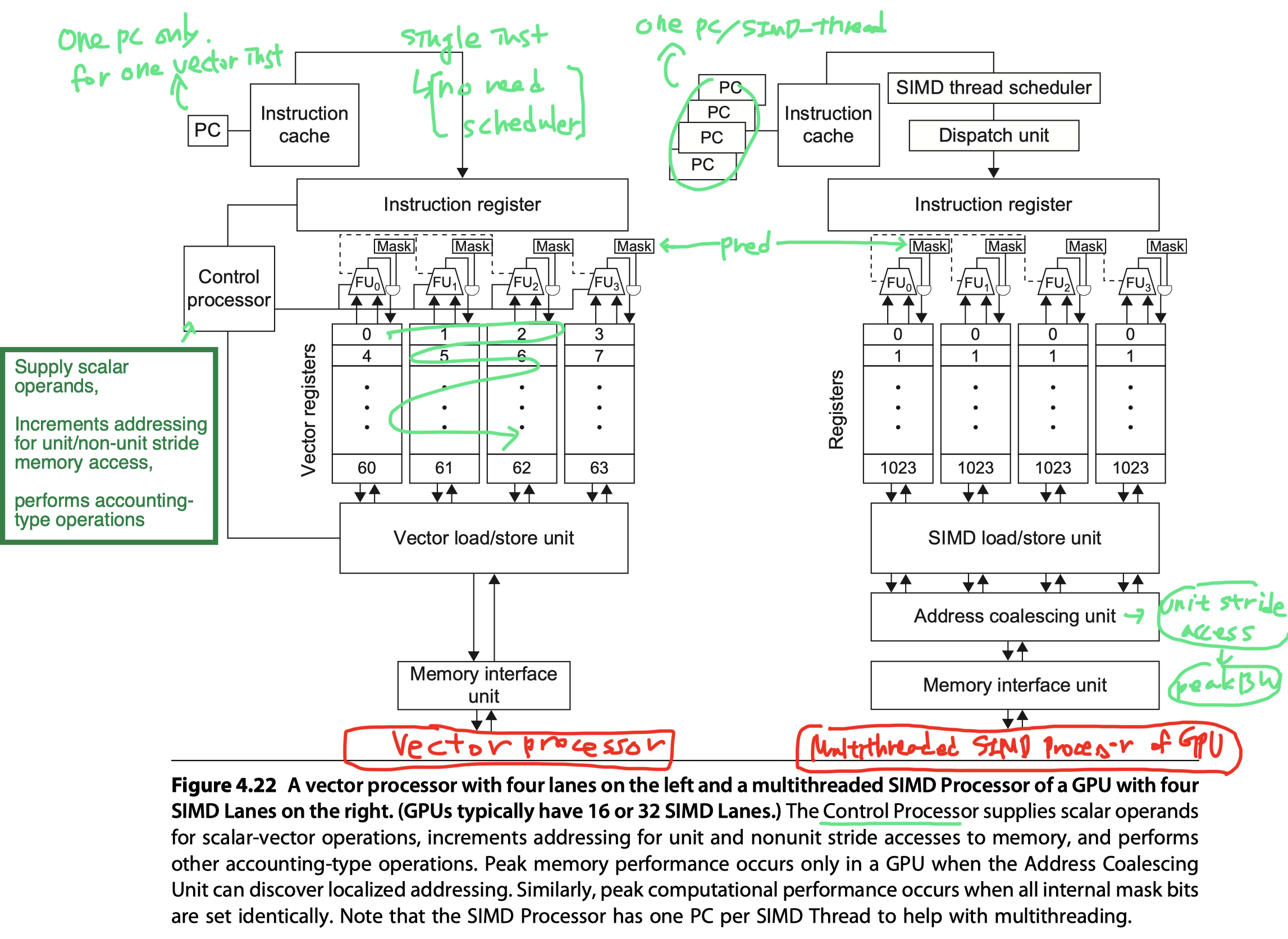
- Control processor of vector computer
- Broadcasts operations to all the Vector Lanes
- Broadcasts a scalar register value for vector-scalar operations
- Does implicit calculations that are explicit in GPUs,
- Such as automatically incrementing memory addresses for
- Unit-stride and
- Nonunit-stride loads and stores
- Such as automatically incrementing memory addresses for
- Missing in the GPU
- Closest analogy in GPU = Thread Block Scheduler
- Assigns Thread Blocks (bodies of vector loop) to multithreaded SIMD Processors
- Runtime hardware mechanisms in a GPU
- Generate addresses
- Discover if they are adjacent (Vector computer don’t need to check. It’s compiler’s job)
- Likely less power-efficient than using a Control Processor
- Scalar processor of vector computer
- Executes the scalar instructions of a vector program
- If too slow to do in the vector unit
- GPU?
- Closest analogy in GPU = System processor
- With thousands of clock cycle overhead
- From the separate address spaces plus transferring over a PCIe bus
- Non-sense to offload scalar operations to the host
- So, just use only one SIMD Lane using the predicate registers for scalar operations! (The other SIMD Lanes are idle.)
- Less efficient than vector architecture
- Closest analogy in GPU = System processor
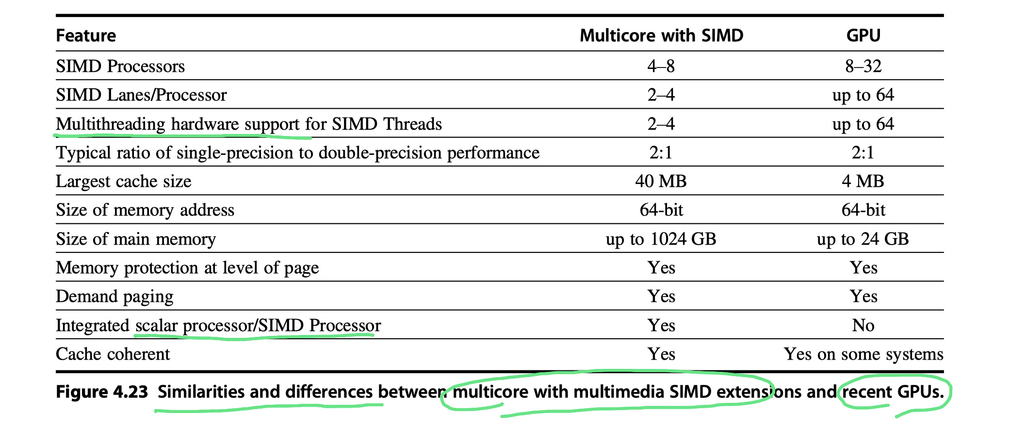
Similarities and Differences Between Multimedia SIMD Computers and GPUs
- GPU share similarities with
- Multicore computers with multimedia SIMD instruction extensions
- Both ..
- Are multiprocessors
- Whose processors use multiple SIMD Lanes
- Use hardware multithreading to improve processor utilization
- Have 2:1 performance ratios between SFP vs DFP
- Use caches
- GPU: Small streaming caches (Put whole working set in the GPU memory)
- Multicore computer: large multilevel caches (Put whole working set in the caches)
- Use a 64-bit address space
- Support memory protection at page
- Are multiprocessors
- Difference?
- SIMD: Not supporting gather-scatter
- And… check Figure 4.23
- Similarity & Numerical difference in processors
Summary
- So GPUs are
- Really just multithreaded SIMD Processors
- More processors, more lanes per processor
- More multithreading hardware than traditional multicore computers
- Less cache memory
- Pascal’s instruction level parallelism
- Issuing instructions from two SIMD Threads to two sets of SIMD Lanes
- CUDA programming model
- Wraps up all these forms of parallelism around a single abstraction, CUDA Thread
- CUDA programmer’s thought
- I’m programming thousands of threads
- In reality,
- The programmer executes each block of 32 threads (or up to 64 SIMD Threads in Pascal P100) on many lanes (eg.64 SIMD Lanes in Pascal P100) of the many SIMD processors (eg. 56 SIMD processors in Pascal P100 )
- So, CUDA programmer should keep in mind for good performance that
- These threads are
- Organized in blocks
- Executed 32 threads at a time
- That addresses need to be to adjacent addresses
- These threads are
- Conversion of terms used in this chapter to NVIDIA, OpenCL, and AMD’ versions
Detecting and Enhancing Loop-Level Parallelism
- This section
- Compiler technology used for discovering the amount of parallelism that we can exploit in a program
- Hardware support for these compiler techniques ?
- Need to define …
- When a loop is parallel (or vectorizable),
- How a dependence can prevent a loop from being parallel
- Techniques for eliminating some types of dependences
- Loop-carried dependence
- Data accesses in later iterations are dependent
- On data values produced in earlier iterations
1
2
3
4
5

for (i=0; i<100; i=i+1) {
	A[i+1] = A[i] + C[i];   /* S1 */
	B[i+1] = B[i] + A[i+1]; /* S2 */
}
// A, B, C are distinct, nonoverlapping arrays
- Two different dependences in the code
- Loop-carried dependence
-
S1(S2) uses a value computed byS1(S2) in an earlier iteration - Forces successive iterations of this loop to execute in series!
-
- Intra-loop dependence
-
S2uses the valueA[i+1]computed byS1in the same iteration - Multiple iteration would execute in parallel
- eg. Sequence of vector instructions that uses chaining
-
- Loop-carried dependence
1
2
3
4

for (i=0; i<100; i=i+1) {
	A[i] = A[i] + B[i];   /* S1 */
	B[i+1] = C[i] + D[i+1]; /* S2 */
}
- What are the dependences between
S1andS2in this code?- Loop-carried dependence between
S2andS1 - But you can make it parallel
- Why? The dependence is not circular
- Key observations to transform the code into a vectorizable loop
- No dependence from
S1toS2- If there were, there would be a cycle in dependences
- So, you can interchange
S1andS2
- On the first iteration,
S2depends on the value ofB[0]computed prior to initiating the loop.
- No dependence from
- Loop-carried dependence between
1
2
3
4
5
6
7

// Code transformation for loop parallelism
A[0] = A[0] + B[0];
for (i=0; i<99; i=i+1) {
	B[i+1] = C[i] + D[i];      /* S2' */
	A[i+1] = A[i+1] + B[i+1];  /* S1' */
}
B[100] = C[99] + D[99];
1
2
3
4

// Recurrence
for (i=1;i<100;i=i+1) {
	Y[i] = Y[i-1] + Y[i];
}
- Recurrence
- A loop-carried dependence when
- A variable is defined based on the value of that variable in an earlier iteration
Finding Dependences
- Complexity of dependence analysis arises because of …
- Presence of arrays and pointers in languages such as C or C++
- Pass-by-reference parameter passing in Fortran
- $\leftrightarrow$ Scalar case is easy
- Scalar variable references explicitly refer to a name,
- They can usually be analyzed quite easily with aliasing
- Nearly all dependence analysis algorithms work on the assumption that
- “Array indices are affine”
- A one-dimensional array index is affine
- If it can be written in the form $a\times i+b$,
- Where
aandbare constants andiis the loop index variable
- The index of a multidimensional array is affine
- If the index of each dimension is affine
- Sparse array accesses?
- Major example of nonaffine accesses
- Typically have form of
x[y[i]]
- Determining whether a dependence between two references to the same array
- = Determining whether two affine functions can have the identical value for different indices between the bounds of the loop.
- Example
- We have stored to an array element with index value $a\times i+b$ and
- Loaded from the same array with index value $c\times i+d$ (eg. matrix transpose),
- Where
iis the for-loop index variable that runs frommton.
- Where
- Dependence exist if two conditions hold:
- (1) $\exists$ two iteration indices, $j$ and $k$, $s.t.$ $m \leq j \leq n$, $m \leq k \leq n$
- (2) Store into an array element indexed by $a\times j+b$
- Later fetches from the same array element when it is indexed by $c\times k+d$
- i.e. $a\times i+b$ = $c\times k+d$
- We cannot determine whether dependence exists at compile time!! Why?
- Sometimes, values of strides (
a,c) and offsets (b,d) are unknown - Compile test for dependence is possible if the variables are constant at compile time
- Sometimes, values of strides (
- Greatest common divisor (GCD) test
- If a loop-carried dependence exists,
- Then GCD (
c,a) must divide (d–b) - Example
- In the code below, a = 2, b=3, c = 2, d = 0
- Then GCD(a,c) = 2, d-b =-3
- 2 does not divide -3
- No dependence is possible
- GCD test is sufficient to guarantee that no dependence exists
- But, $\exists$ cases where GCD test succeeds, but no dependence exists
- Because GCD test does not consider the loop bounds
1
2
3
4

//Example of GCD test
for (i=0; i<100; i=i+1){
	X[2*i+3] = X[2*i] * 5.0;
}
- Determining whether a dependence actually exists is NP-complete.
- However, in practice, possible to detect at low cost
- Recently, using a hierarchy of exact tests is accurate and efficient
- Need to classify the type of dependence as well
- In addition to determining the existence of dependence
- To recognize name dependences and
- Eliminate them at compile time by
- Renaming and
- Copying
1
2
3
4
5
6

for (i=0; i<100; i=i+1) {
	Y[i] = X[i] / c; /* S1 */
	X[i] = X[i] + c; /* S2 */
	Z[i] = Y[i] + c; /* S3 */
	Y[i] = c - Y[i]; /* S4 */
}
- Dependences in this code
- (1) True dependences
- From
S1toS3forY[i] - From
S1toS4forY[i]
- From
- (2) Antidependence
- From
S1toS2, based onX[i] - From
S3toS4forY[i]
- From
- (3) Output dependence
- From
S1toS4, based onY[i]
- From
- (1) True dependences
1
2
3
4
5
6
7
8
9
10

// A version of the loop that eliminates these false (or pseudo) dependences
for (i=0; i<100; i=i+1 {
	// Y renamed to T to remove output dependence
	T[i] = X[i] / c;
	// X renamed to X1 to remove antidependence
	X1[i] = X[i] + c;
	// Y renamed to T to remove antidependence
	Z[i] = T[i] + c;
	Y[i] = c - T[i];
}
- The major drawback of dependence analysis
- It applies only under a limited set of circumstances
- Namely, among references within a single loop nest and using affine index functions
- There are many situations where array-oriented dependence analysis cannot tell us what we want to know;
- For example, analyzing accesses done with pointers, rather than with array indices can be much harder.
- = One reason why Fortran is still preferred over C and C++ for many scientific applications designed for parallel computers
- Analyzing references across procedure calls is extremely difficult
- Need approaches as OpenMP and CUDA that
- Write explicitly parallel loops
- It applies only under a limited set of circumstances
Eliminating Dependent Computations
- One of the most important forms of dependent computations is a recurrence
1
2
3
4
5
6
7
8
9
10
11
12
13
14
15
16
17
18
19

for (i=9999; i>=0; i=i-1)
	sum = sum + x[i] * y[i];
// => Loop-carried depedendence on "sum"

// How to eleiminate the denpendence?
// => Transform it to a set of loops
// "Scalar exepansion" on "sum"
for (i=9999; i>=0; i=i-1) // Loop #1
		sum[i] = x[i] * y[i];

// Not parallel, but a very specific structure called "reduction", which is common in linear algebra & a key part of the primary primative "MapReduce".
for (i=9999; i>=0; i=i-1) // Loop #2
	finalsum = finalsum + sum[i];

// If you parallelsize the reduction with multiple processors indexed by "p", and complete it by multiple steps
for (i=999; i>=0; i=i-1)
	finalsum[p] = finalsum[p] + sum[i+1000*p];

// And then finally reduce the much small size finalsum vector to a output scalar
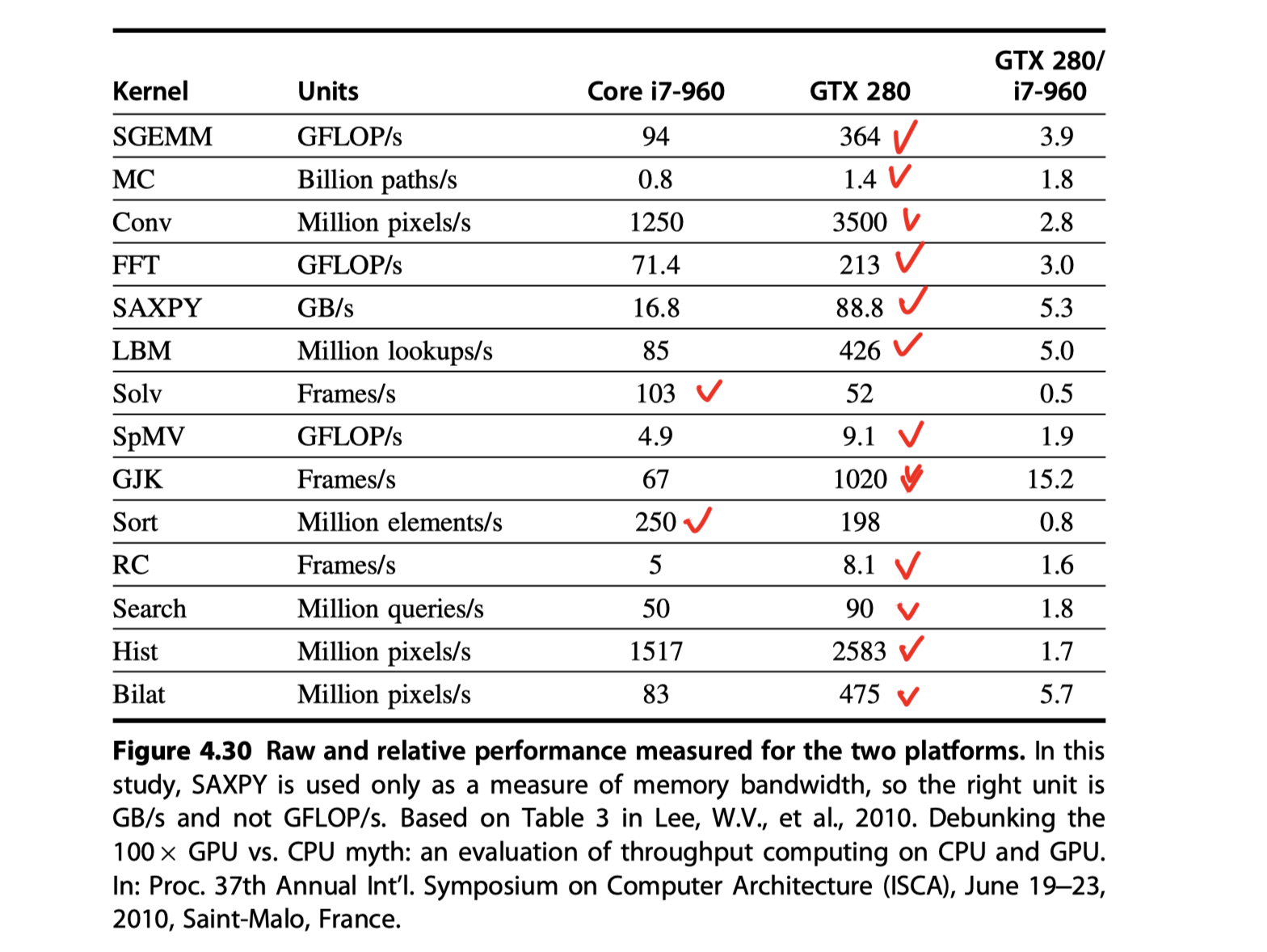
Putting It All Together: CPU vs GPU
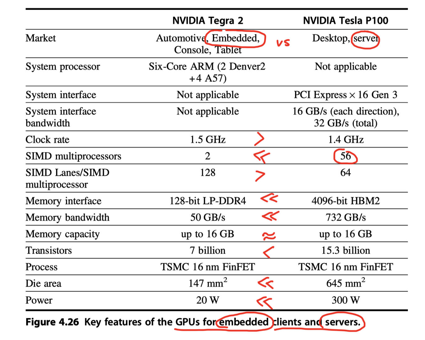
-
Embedded GPU vs Server GPU
-
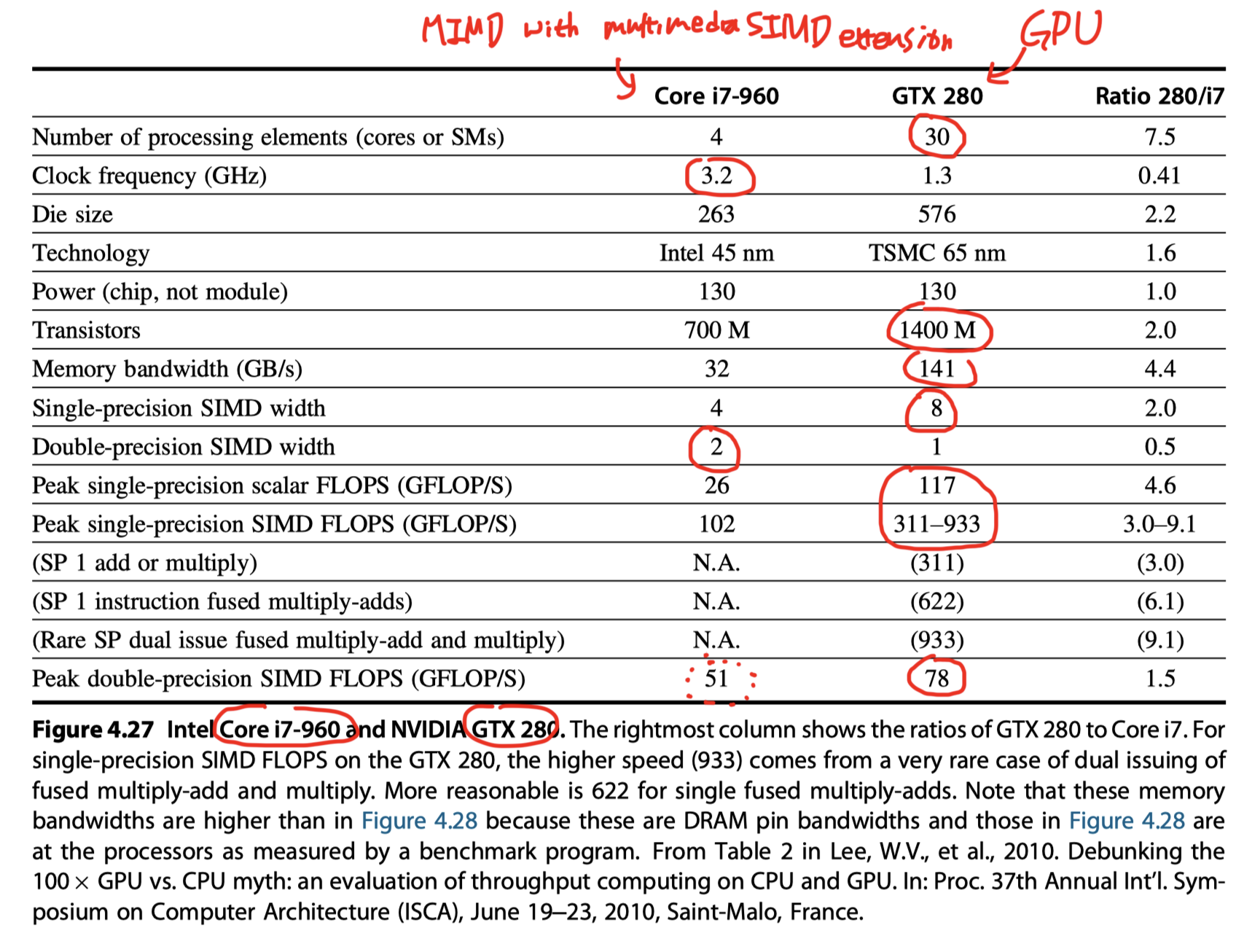
MIMD with SIMD extension vs GPU
-
Roofline
Reference
- Chapter 4 in Computer Architecture A Quantitative Approach (6th) by Hennessy and Patterson (2017)
- Notebook: Computer Architecture Quantitive Approach
- Do CUDA threads execute in lockstep for O(n) operations? from StackOverfLow
- Vector Processor-Encyclopedia, Science News & Research Reviews
- Vector processor working - Example of a simple vectorized loop execution
Notes Mentioning This Note
Table of Contents
- Data-Level Parallelism in Vector, SIMD, and GPU Architectures
- Introduction
-
Vector Architecture
- RV64V Extension
- How Vector Processors Work: An Example
- Vector Execution Time
- Multiple Lanes: Beyond One Element per Clock Cycle
- Vector-Length Registers: Handling Loops Not Equal to 32
- Predicate Registers: Handling IF Statements in Vector Loops
- Memory Banks: Supplying Bandwidth for Vector Load/Store Units
- Stride: Handling Multidimensional Arrays in Vector Architectures
- Strided Accesses and TLB Misses in Cross-Cutting Issues
- Gather-Scatter: Handling Sparse Matrices in Vector Architectures
- Programming Vector Architectures
- SIMD Instruction Set Extensions for Multimedia
-
Graphics Processing Units
- Programing the GPU
- NVIDIA GPU Computational Structures
- NVIDIA GPU Instruction Set Architecture
- Conditional Branching in GPUs
- NVIDIA GPU Memory Structures
- Innovations in the Pascal GPU Architecture
- Similarities and Differences Between Vector Architectures and GPUs
- Similarities and Differences Between Multimedia SIMD Computers and GPUs
- Summary
- Detecting and Enhancing Loop-Level Parallelism
- Putting It All Together: CPU vs GPU
- Reference