Instruction-Level Parallelism and Its Exploitation
- Chapter 3 in Computer Architecture A Quantitative Approach (6th) by Hennessy and Patterson (2017)
Instruction-Level Parallelism: Concepts and Challenges
-
Instruction-level parallelism (ILP)
- All processors since about 1985 $\rightarrow$ Pipelining to overlap the instruction execution
- Appendix C: Basic pipelining in Pipelining Basic and Intermediate Concepts
- This chapter + appendix H: More advanced level
- Largely separable approaches to exploiting ILP
-
Hardware to help discover and exploit the parallelism dynamically
- All Intel/ARM processors
- IOT $\rightarrow$ Lower level of ILP
-
Software technology to find parallelism statically at compile time
- Limited to domain-specific environments
- Scientific applications
- Data-level parallelism
-
Hardware to help discover and exploit the parallelism dynamically
-
ILP limitation $\rightarrow$ Movement toward “multicore”
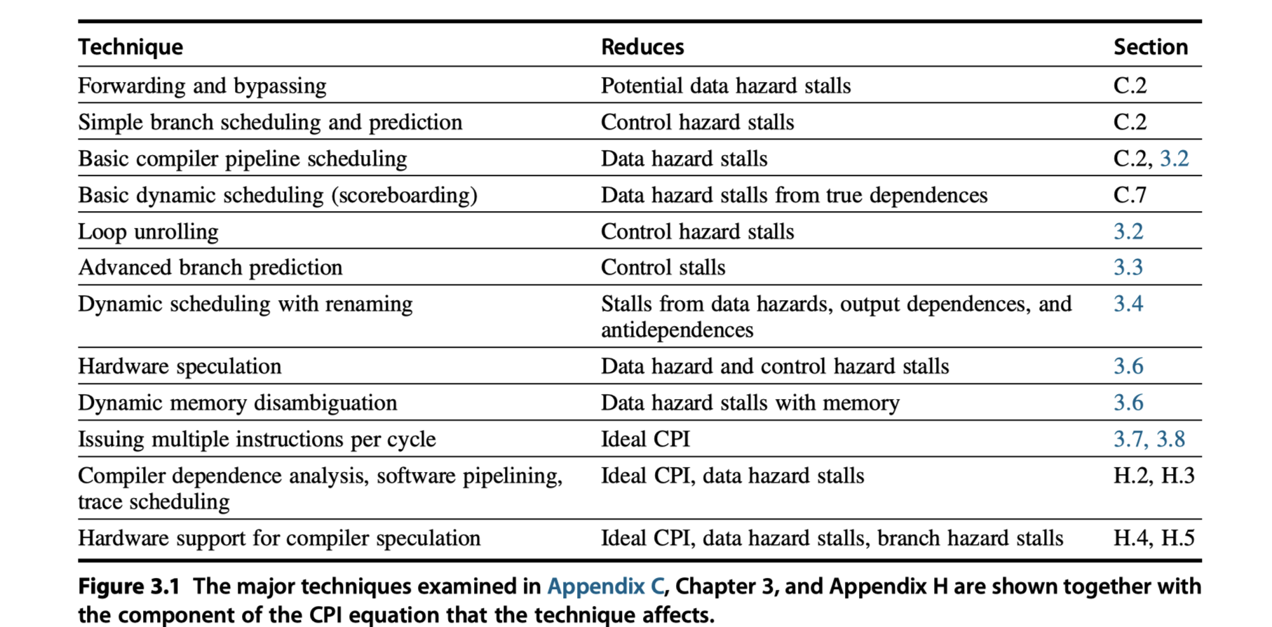
- Pipeline CPI = Ideal pipeline CPI + Structural stalls + Data hazard stalls + Control stalls
What is Instruction-Level Parallelism?
- The amount of parallelism
- Available within a basic block is quite small.
- Basic block: a straight-line code sequence with no branches in except to the entry and no branches out except at the exit
- More dependency within a basic block
- 15% ~ 25% branch frequency
-
So, we must exploit ILP across multiple basic blocks
-
Loop-level parallelism into ILP
- Unrolling the loop either statically by the compiler
- Dynamically by the hardware
-
Loop-level parallelism into Data-parallelism in Chapter 4:
- The use of SIMD in both vector processors and graphics processing units (GPUs)
- Vector instruction using parallel execution and deep pipeline
1
2

for (i=0; i<=999; i++)
	x[i] = x[i] + y[i];
- Example code
- Seven instructions per iteration
- 2 loads, 1 add, 1 store, 2 address updates, and a branch
- 7000 instructions in total
- 1800 (1/4x) using SIMD architecture instructions ~
-
Only 4 instructions using some vector processors
- 2 vector loads
- 1 vector add
- 1 vector store
- Seven instructions per iteration
Data Dependences and Hazards
-
How one instruction depends on another??
- If two instructions are
- Parallel $\rightarrow$ Execute simultaneously
- Dependent $\rightarrow$ Must be executed in order
- Three different types of dependences
- Data dependences (True data dependences)
- Name dependences (Not-true data dependences)
- Control dependences
True Data Dependences
(Read-After-Write)
- Instruction $j$ is data-dependent on instruction $i$ if …
- $i$ produces a result that may be used by $j$ … or …
- $j$ is data-dependent on $k$, $k$ is dependent on $i$
- Chain of dependences of the first type
- If two instructions are data-dependent
- Must execute in order
- Cannot execute simultaneously
- Then, a processor …
- With pipeline interlocks $\rightarrow$ Detect a hazard and stall
- Without pipeline interlocks $\rightarrow$ Rely on compiler scheduling
- $\rightarrow$ Not completely overlapped schedule
-
Three limitation from data dependence
- (1) The possibility of a hazard
- (2) The order in which results must be calculated
- (3) An upper bound on how much parallelism can possibly be exploited.
- How to overcome the limitations?
- (1) Maintaining the dependence but avoiding a hazard
- (2) Eliminating a dependence by transforming the code
- $\rightarrow$ Scheduling by the hardware or the compiler
- Data value may flow between instructions either …
-
Through registers
- Detecting the dependence is straightforward
- Check register names!
-
Through memory locations
- More difficult to detect
- Why?
- Two address may refer to the same location but look different
- eg. It’s possible that 100(x4) == 20(x6)
- Or, the effective address may change from one execution of the instruction to another
- eg. 20(x4) in $i$ and 20(x4) in $j$ may be different
- Two address may refer to the same location but look different
-
Through registers
Name Dependences
-
Two instructions use the same register or memory location, called a name, but there is no flow of data between the instructions associated with that name
-
Two types of name dependences ($i$ precedes $j$)
-
Antidependence
- $j$ writes a register or memory location that $i$ reads
- The original ordering must be preserved to ensure that $i$ reads the correct value (WAR)
- eg.
fsdandaddion registerx1
-
Output dependence
- $i$ and $j$ write the same register or memory location
- The ordering between the instructions must be preserved to ensure that the value finally written corresponds to $j$ (WAW)
- Both are not true dependences
- No value being transmitted between the instructions
- Change the name ! $\rightarrow$ Then, you can execute simultaneously or reorder the instructions!!
- More easy for register operands than memory locations $\rightarrow$ Register renaming
-
Antidependence

Data Hazards (True + Name)
- Exploit parallelism by preserving program order
- Only where it affects the outcome of the program.
-
Detecting and avoiding hazards ensures
- that necessary program order is preserved.
- Possible data hazards
- RAW ($j$ read after $i$ write)
- WAW ($j$ write after $i$ write)
- WAR ($j$ write after $i$ read)
Control Dependences
-
A control dependence determines the ordering of an instruction, $i$, with respect to a branch instruction so that instruction $i$ is executed in correct program order and only when it should be
-
One of the simplest examples of a control dependence
- The dependence of the statements in the “then” part of an if statement on the branch.
-
S1is control-dependent onp1 -
S2is control-dependent onp2but not on p1
1
2
3
4
5
6

if p1 {
	S1;
};
if p2 {
	S2;
}
- Two constraints imposed by control dependences:
- (1) An instruction that is control-dependent on a branch cannot be moved before the branch
- Don’t move the instructions in
thenstatement before itsifstatement
- Don’t move the instructions in
- (2) An instruction that is not control-dependent on a branch cannot be moved after the branch so that its execution is controlled by the branch.
- Don’t move the instructions in the statements before
ifstatement tothenstatement
- Don’t move the instructions in the statements before
- (1) An instruction that is control-dependent on a branch cannot be moved before the branch
- Control dependence is not the critical property that must be preserved.
- You can violate the control dependences, if you can do so without affecting the correctness of the program
- Two properties critical to program correctness—and normally preserved by maintaining both data and control dependences—are …
- (1) the exception behavior and
- (2) the data flow.
-
(1) Preserving the exception behavior?
- Any changes in the ordering of instruction execution must not change how exceptions are raised in the program.
- Relaxed version: The reordering of instruction execution must not cause any new exceptions in the program.
-
add$\leftrightarrow$beq: Don’t maintain data dependence?- $\rightarrow$ Change the result
-
beq$\leftrightarrow$ld: Don’t maintain control dependence?- $\rightarrow$ Cause a memory protection exception
- If you still want to reorder?
- Just ignore the exception when the branch is taken
- Speculation technique overcome this exception problem
- Appendix H: Software techniques for supporting speculation
	add x2, x3, x4
	beq x2, x0, L1
	ld x1, 0(x2)
L1:
-
(2) Preserving the dataflow?
- Dataflow : The actual flow of data values among instructions that produce results and those that consume them.
- Branches make the dataflow dynamic because they allow the source of data for a given instruction to come from many points
-
add/ordata dependence is depending on whether the branch is taken or not -
orinstruction has data dependence on bothaddandsub, but depending on the branch - So, preserve the control dependence of the
oron the branch!!
	add x1, x2, x3
	beq x4, x0, L
	sub x1, x5,x6
L:  ...
    or x7, x1, x8
- Sometimes we can determine that violating the control dependence cannot affect either the exception behavior or the dataflow
-
x4insubwill be unused (dead) afterskiplabel - Move
subbefore the branch - The dataflow could not be affected!!
- a.k.a. software speculation
- The compiler is betting on the branch outcome; in this case, the bet is that the branch is usually not taken
-
	add x1,x2,x3
	beq x12,x0,skip
	sub x4,x5,x6
	add x5,x4,x9
skip: or x7,x8,x9
- Control dependence is preserved by implementing hazard detection that causes control stalls
Basic Compiler Techniques for Exposing ILP
- This section examines the use of simple compiler technology to enhance a processor’s ability to exploit ILP
- Appendix H will investigate more sophisticated compiler and associated hardware schemes designed to enable a processor to exploit more instruction-level parallelism
Basic Pipeline Scheduling and Loop Unrolling
- Keep a pipeline full?
- $\rightarrow$ Find sequences of unrelated instructions that can be overlapped in the pipeline!
-
Separate the execution of a dependent instruction
- From the source instruction
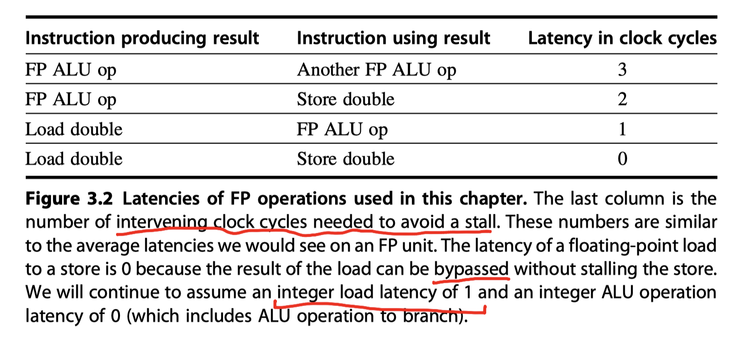
- By a distance in clock cycles
- Equal to the pipeline latency of that source instruction.
- How the compiler can increase the amount of available ILP by transforming loop?
1
2
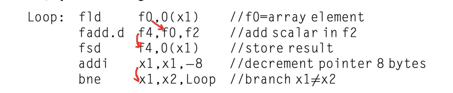
for (i=999; i>=0; i=i-1)
x[i] = x[i] + s;
-
Translated to RISC-V code

-
Clock cycle issued?

- Move
addiup to fill the first stall- Gain? 8 cycles $\rightarrow$ 7 cycles
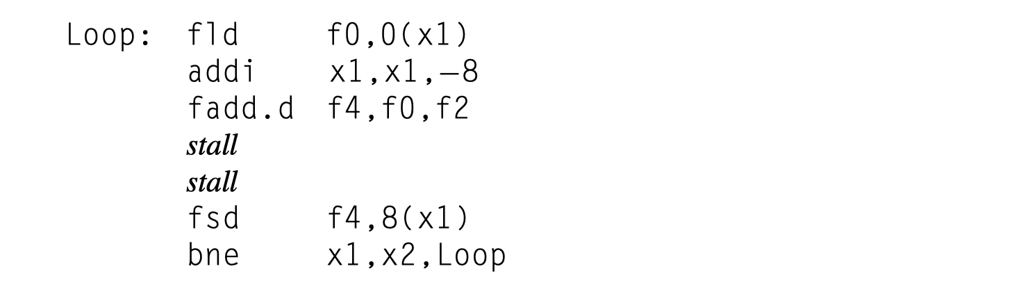
- Gain? 8 cycles $\rightarrow$ 7 cycles
-
Now, the remaining four clock cycles consist of loop overhead—the
addiandbneand two stalls. -
Loop unrolling
- Unrolling simply replicates the loop body multiple times,
- Adjusting the loop termination code
- Unroll four copies of the loop body in a loop
- Eliminated three branches and three decrements of
x1 - 8 cycles per element $\rightarrow$ 6.5 cycles per element
- Requires symbolic substitution and simplification
- General forms of theses optimization in Appendix H
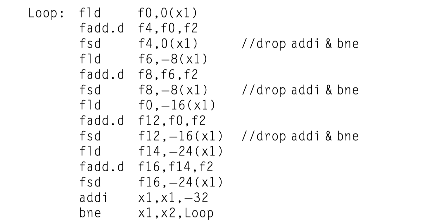
- Eliminated three branches and three decrements of
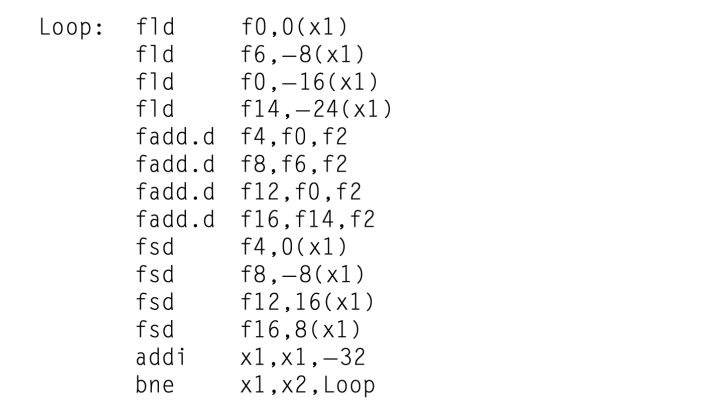
- Unrolling followed by scheduling?
- Original code: 8 cycles per element
- Unrolled, not scheduled: 6.5 cycles per element
- Unrolled, and scheduled: 3.5 cycles per element (No stall!)
- Gain on the unrolled loop is even larger than the original loop!
Summary of the Loop Unrolling and Scheduling
- The key to most of these techniques is to know when and how the ordering among instructions may be changed
- This process must be performed in a methodical fashion either by a compiler or by hardware.
- To obtain the final unrolled code,
- Determine that unrolling the loop would be useful by finding that the loop iterations were independent, except for the loop maintenance code.
- Use different registers to avoid unnecessary constraints that would be forced by using the same registers for different computations (e.g., name dependences).
- Eliminate the extra test and branch instructions and adjust the loop termination and iteration code.
- Determine that the loads and stores in the unrolled loop can be interchanged by observing that the loads and stores from different iterations are independent. This transformation requires analyzing the memory addresses and finding that they do not refer to the same address.
- Schedule the code, preserving any dependences needed to yield the same result as the original code.
- The key requirement:
- How one instruction depends on another and how the instructions can be changed or reordered given the dependences.
- Limit the gains from loop unrolling?
- (1) A decrease in the amount of overhead amortized with each unroll
- (2) code size limitations
- (3) compiler limitations
- The potential shortfall in registers = “register pressure”
Reducing Branch Costs With Advanced Branch Prediction
- Loop unrolling $\rightarrow$ Reduce # branch hazards
- Also reduce the performance losses of branches by predicting how they will behave
- Simple branch predictors $\rightarrow$ Appendix C summarized in Pipelining Basic and Intermediate Concepts
- # instructions in flight $\uparrow$ with deeper pipelines and more issues per clock
- $\rightarrow$ Need more accurate branch prediction !
Correlating Branch Predictors
- The 2-bit predictor in Appendix C (See Pipelining Basic and Intermediate Concepts)
- Use only the recent behavior of a single branch
- Possible to improve the prediction accuracy if we also look at the recent behavior of other branches
- A C code fragment from the
eqntottbenchmark1 2 3 4 5 6 7
if (aa==2) aa=0; if (bb==2) bb=0; if (aa!=bb) { ... }
-
RISC-V code version
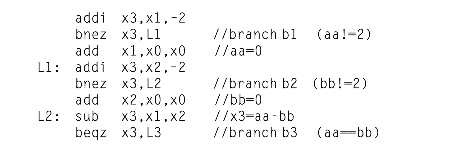
- Key observation of the code
- The behavior of branch
b3is correlated with the behavior of branchesb1andb2 - If neither
b1norb2are taken,b3will be taken
- The behavior of branch
-
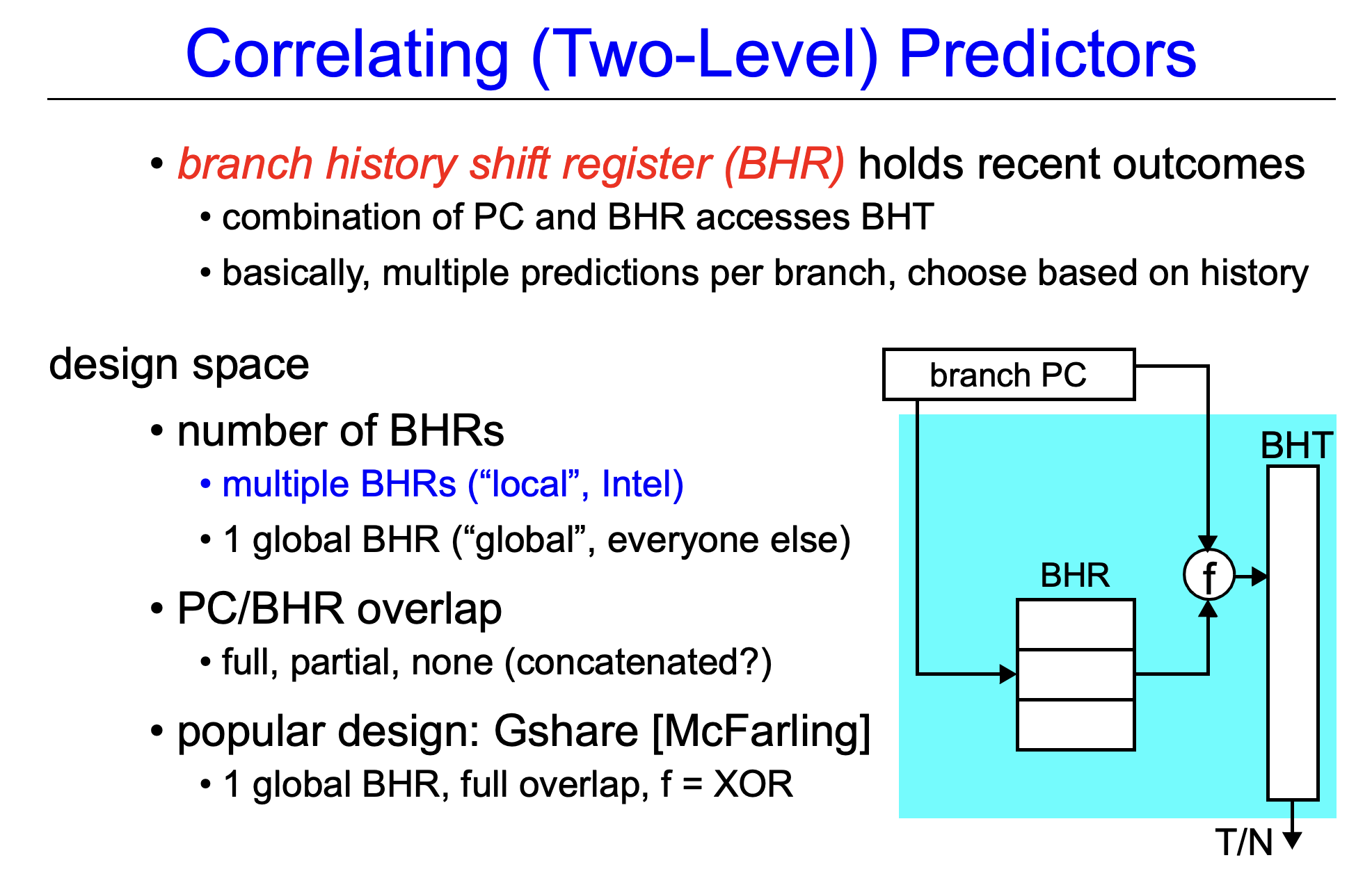
Correlating predictors or Two-level predictors
- Branch predictors that use the behavior of other branches to make a prediction
- (m,n) predictor uses the behavior of the last m branches to choose from $2^m$ branch predictors, each of which is an n-bit predictor for a single branch
- Higher prediction rates than the 2-bit scheme and requires only a trivial amount of additional hardware
- Simplicity of the hardware?
- m-bit shift register records the global history of the most recent $m$ branches (eg. 0 for taken, 1 for not-taken)
- The branch-prediction buffer (or table) can then be indexed using a concatenation of the low-order bits from the branch address with the m-bit global history
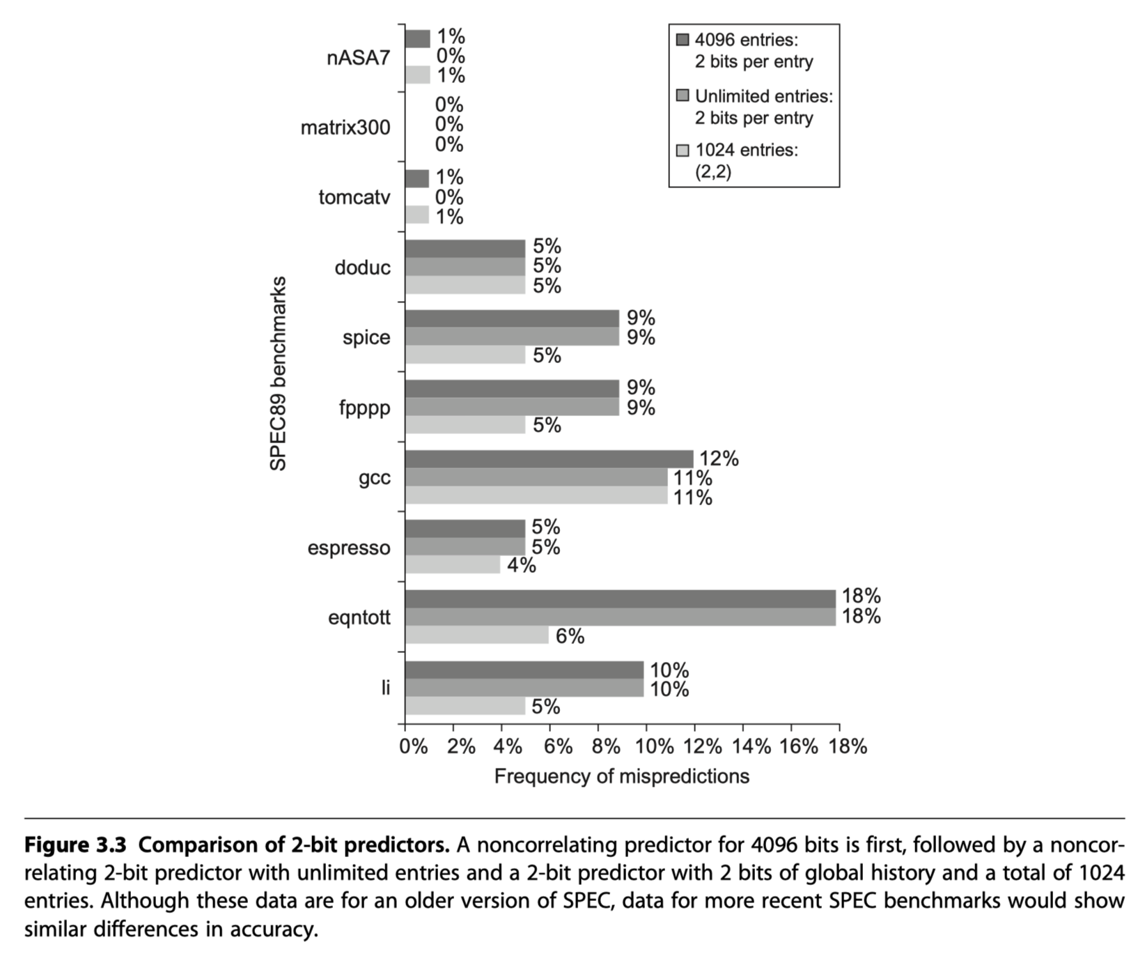
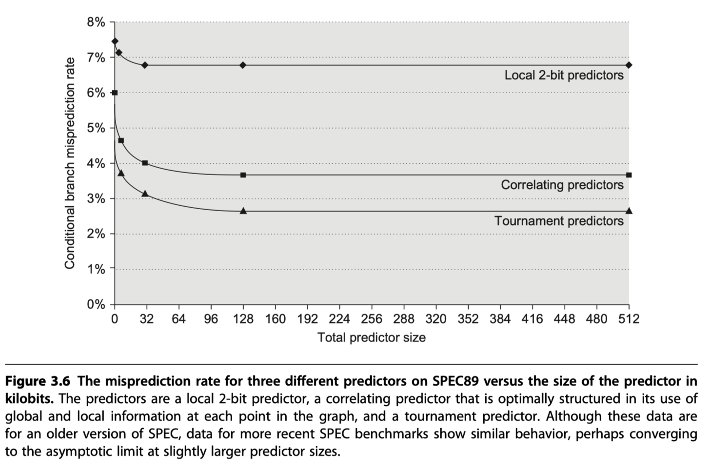
- Comparisons of 2bit predictors
- Non-correlating 2bit predictors with 4096 entries
- vs (2,2) correlating predictors with 1024 entries
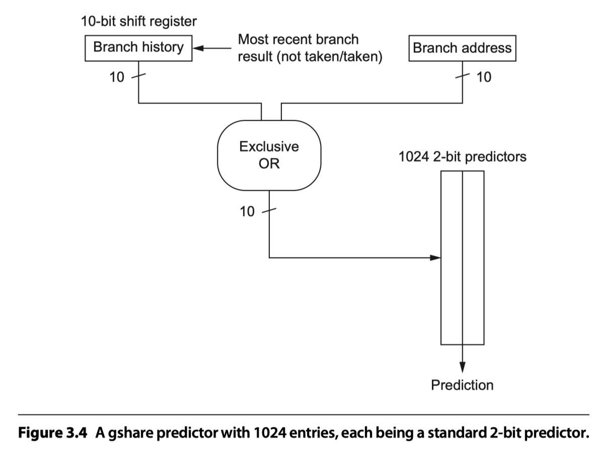
- The best-known example = McFarling’s gshare predictor
- Index = Combining the address of the branch and most recent branch outcomes using exclusive OR
- i.e. Hashing the branch address and the branch history
Tournament Predictors: Adaptively Combining Local and Global Predictors
- Use both a global predictor and a local predictor
- Global predictor’s index = branch address + global branch history
- Local predictor’s index = branch address
- Choose between them with a selector
- eg. 2-bit saturating counter per branch to choose among two different predictors (local vs global)
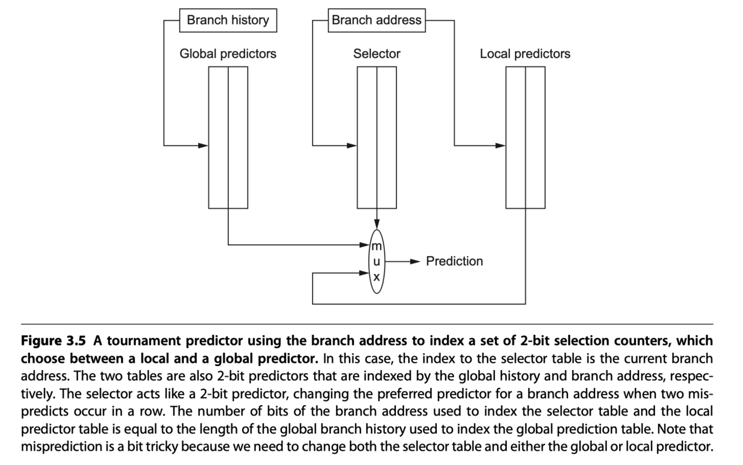
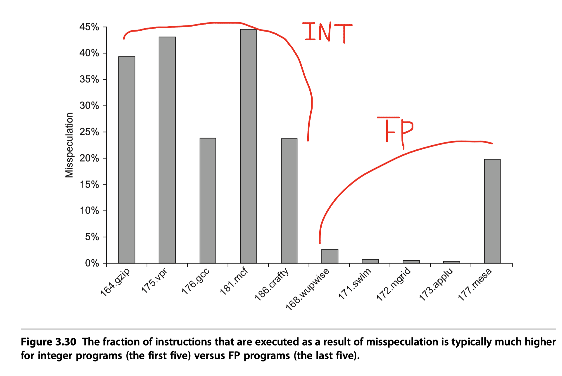
- Typically select the global predictor
- ~ 40% for SPEC integer benchmarks
- < 15% for SPEC FP benchmarks
- Used in Alpha processors and several AMD processors
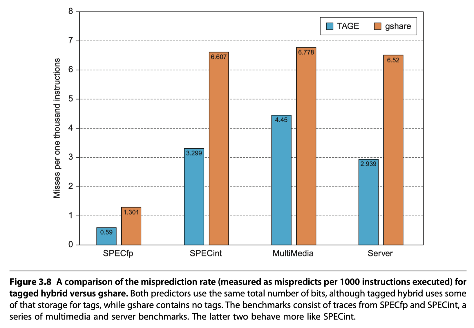
Tagged Hybrid Predictors
- The best branch prediction scheme as of 2017!!
- Combining multiple predictors that track whether a prediction is likely to be associated with the current branch.
-
Tagged hybrid predictors (Seznec and Michaud, 2006)
- Loosely based on an algorithm for statistical compression called PPM (Prediction by Partial Matching)
- PPM attempts to predict future behavior based on history
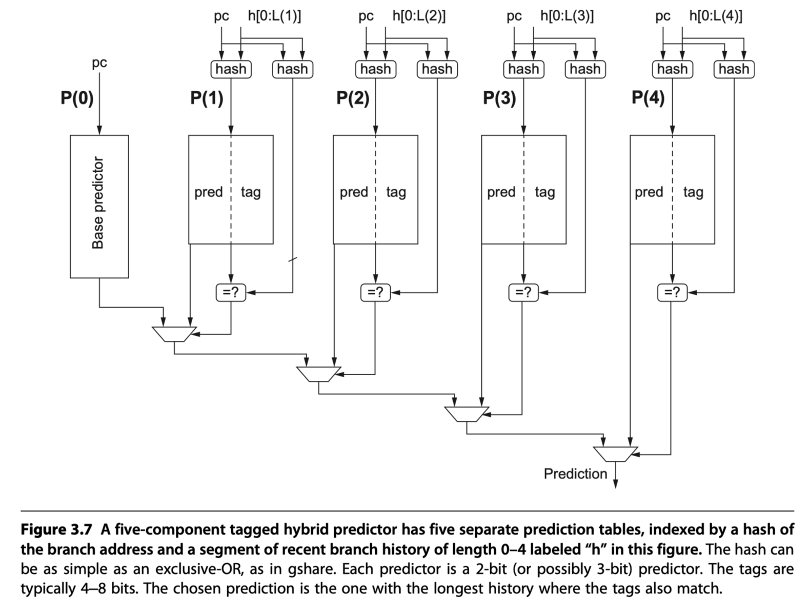
- Five-component tagged hybrid predictor
-
Five prediction table:
P(0), …P(4)-
P(i)is accessed using a hash of the PC and the history of the most recent $i$ branches (kept in a shift register) - i.e Use multiple history lengths from 0 to i !
-
- Use tags in tables
P(1)throughP(4)- 100% matches are not required $\rightarrow$ Short tag! (Allow a little bit of inaccuracy)
- A small tag of 4-8 bits appears to gain most of the advantage
- A prediction from P(1), . . . P(4) is used only if the tags match the hash of the branch address and global branch history
- Each of the predictors = 2-bit or 3-bit counter
-
P(0)= default predictor
-
Five prediction table:
-
Tagged hybrid predictors (TAGE: TAgged GEometic predictors) and the earlier PPM-based predictors $\rightarrow$ The winners in recent annual international branch-prediction competitions
- Initializing predictors : Use “hint bits” so that the predictors give accurate result in the initial stage with little prediction history
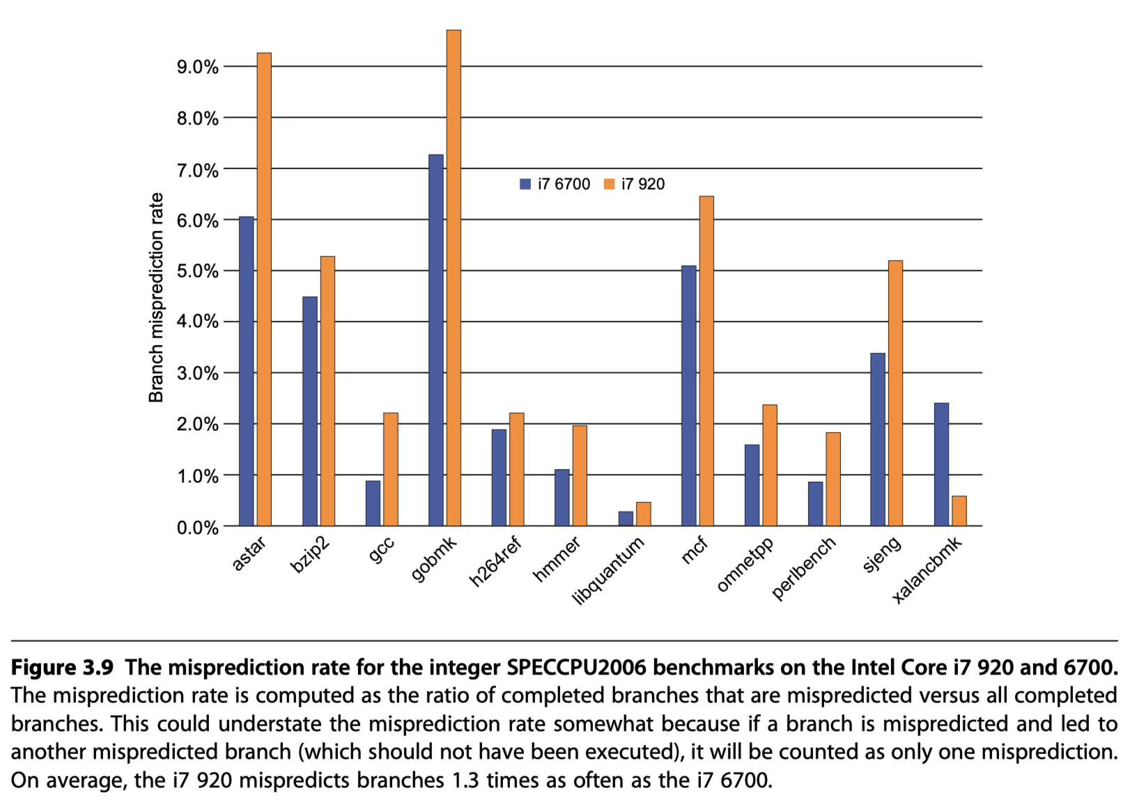
The Evolution of the Intel Core i7 Branch Predictor
- Six generations of Intel Core i7 processors between 2008~2016
- Deep pipelining
- Multiple issues per clock
- Many instructions in-flight at once
- up to 256 !!
- at least 30 !!
- This makes branch prediction critical !!
- Secret !!
-
Core i7 920’s branch predictor
-
Two-level predictor
- a smaller first-level predictor
- a larger second-level predictor as a backup
- Each predictor
- (1) Simple 2-bit predictor
- (2) Global history predictor
- (3) Loop exit predictor
- Uses a counter to predict the exact number of taken branches (=#loop iteration) for a loop branch
- A separate unit predicts target addresses for indirect branches
- A stack to predict return address
-
Two-level predictor
- The newest i7 processors?
- Maybe using a tagged hybrid predictor
- Combines the functions of all three second-level predictors in earlier i7
Overcoming Data Hazards With Dynamic Scheduling
-
Dynamic scheduling
- The hardware reorders the instruction execution to reduce the stalls while maintaining data flow and exception behavior
- Advantages
- (1) Eliminating the need to have multiple binaries and recompile for a different microarchitecture
- (2) Enables handling some cases when dependences are unknown at compile time
- (3) Tolerate unpredictable delays, such as cache misses, by executing other code while waiting for the miss to resolve
-
At the cost of a significant increase in hardware complexity!!
- Dynamic vs Static scheduling?
- Static: Minimize data dependences (by separating dependent instructions)
- Dynamic: Avoid stalling when dependences are present
Dynamic Scheduling: The Idea
- If instruction $j$ depends on a long-running instruction $i$ $\rightarrow$ $j$ must be stalled
fdiv.d f0,f2,f4
fadd.d f10,f0,f8
fsub.d f12,f8,f14
-
fsub.dcannot execute- Because of the dependence of
fadd.donfdiv.d(RAW) - But,
fsub.ditself is NOT data-dependent!
- Because of the dependence of
-
Can we execute
fsub.dwithout stall? - In-order pipeline
- Both structural and data hazards are checked during instruction decode (ID)
- If no structural/data hazards, issued from ID
- Out-of-order execution (i.e. Out-of-order completion)
-
Separate the issue process into two parts!
- (1) Checking for any structural hazards
- (2) Waiting for the absence of a data hazard
- $\rightarrow$ We still use in-order instruction issue = Issued in program order
-
- But, begin execution as soon as its data operands are available!
-
Separate the issue process into two parts!
- Possibility of WAR and WAW hazards in OoO exeuction
- Does not exist in in-order pipeline
- eg. An antidependence between
fmul.dandfadd.dforf0- if
fadd.dis executed beforefmul.d(which is waiting forfdiv.d) - Violate the antidependence, yielding a WAR hazard
- if
- $\rightarrow$ Avoided by the use of register renaming
fdiv.d f0,f2,f4
fmul.d f6,f0,f8
fadd.d f0,f10,f14
- Must preserve exception behavior
- Exactly those exceptions that would arise if the program were executed in strict program order actually do arise.
- How? Delay the notification of an associated exception until the processor knows that the instruction should be the next one completed.
- Could generate imprecise exception
- i.e. the processor state (when an exception is raised) does not look exactly as if the instructions were executed sequentially in strict program order.
- $\rightarrow$ Difficult to restart execution after an exception
- Case1) The pipeline may have already completed instructions that are later in program order than the instruction causing the exception.
- Case2) The pipeline may have not yet completed some instructions that are earlier in program order than the instruction causing the exception.
- $\rightarrow$ Solution in Section 3.6, Appendix J
-
Splitting the ID pipe stage of our simple five-stage pipeline into two stages
- (1) Issue: Decode instructions, check for structural hazards.
- (2) Read operands: Wait until no data hazards, then read operands.
- Distinguish
- When an instruction begins execution and
- When it completes execution
- Execution in between the two times
- Allow multiple instructions to be in execution at the same time
- Multiple functional units
- Pipelined function units
- Or Both
-
Dynamically scheduled pipeline
- Pass through the issue stage in order (in-order issue)
- Stalled/Bypass each other in the second stage (read operands)
- Enter execution out of order
-
Scoreboarding
- Allows instructions to execute out of order when there are
- sufficient resources (no structural hazard) and
- no data dependences (no data hazard)
- Allows instructions to execute out of order when there are
- More developed technique = Tomasulo’s algorithm
- Handle anti-dependences and output dependences
- By renaming the registers dynamically
- Can be extended to handle speculation
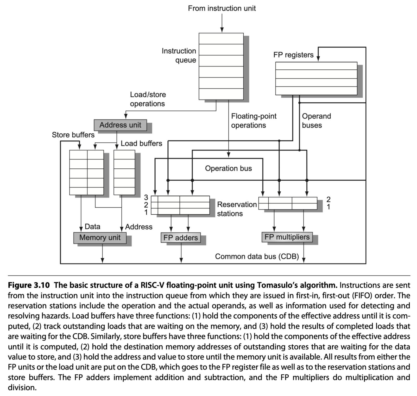
Dynamic Scheduling Using Tomasulo’s Approach
-
Robert Tomasulo’s scheme used in IBM 360/91 floating-point unit
- (1) Tracks when operands for instructions are available to minimize RAW hazards $\in$ Scoreboarding
- (2) Introduces register renaming in hardware to minimize WAW and WAR hazards.
- Two key principles:
- (1) Dynamically determining when an instruction is ready to execute
- (2) Renaming registers to avoid unnecessary hazards
- Motivation?
- IBM360 had only 4 DP registers $\rightarrow$ Limited the effectiveness of compiler scheduling
- IBM360’s long memory accesses and long FP delays
- Overlapped execution of multiple iterations of a loop
-
Register renaming?
- Eliminate WAR/WAW hazards
- By renaming all destination registers
- With a pending read or write for an earlier instruction
- So the OoO write does not affect any instructions that depend on an earlier value of an operand
fdiv.d f0,f2,f4
fadd.d f6,f0,f8
fsd f6,0(x1)
fsub.d f8,f10,f14
fmul.d f6,f10,f8
- Three true data dependence $\rightarrow$ RAW
-
fdiv.d&fadd.d -
fsub.d&fmul.d -
fadd.d&fsd
-
- Two anti-dependences $\rightarrow$ WAR
-
fadd.dandfsub.donf8 -
fsdandfmul.donf6
-
- Output dependence $\rightarrow$ WAW
-
fadd.dandfmul.donf6
-
- The three anti-/output dependence $\rightarrow$ Eliminated by register renaming
- Assume two temporary registers, S & T
fdiv.d f0,f2,f4
fadd.d S,f0,f8
fsd S,0(x1)
fsub.d T,f10,f14
fmul.d f6,f10,T
-
Reservation stations
- Provide register renaming in Tomasulo’s scheme
- Buffer the operands of instructions waiting to issue
- Fetches and buffers an operand as soon as it is available
- Eliminating the need to get the operand from a register
- Pending instructions designate the reservation station that will provide their input
- When successive writes to a register overlap in execution
- $\rightarrow$ Only the last one is actually used to update the register.
- As instructions are issued, the register specifiers for pending operands are renamed to the names of the reservation station, which provides register renaming.
- More reservation stations than real registers $\rightarrow$ Even eliminate hazards due to name dependences
- Two properties of Tomasulo’s scheme
- (1) Hazard detection and execution control are distributed
- Reservation stations are attached to each functional unit
- (2) Results from the reservation stations (Not from registers) $\rightarrow$ directly to functional units
- Bypassing is done with a common result bus (common data bus, CDB on the 360/91)
- (1) Hazard detection and execution control are distributed
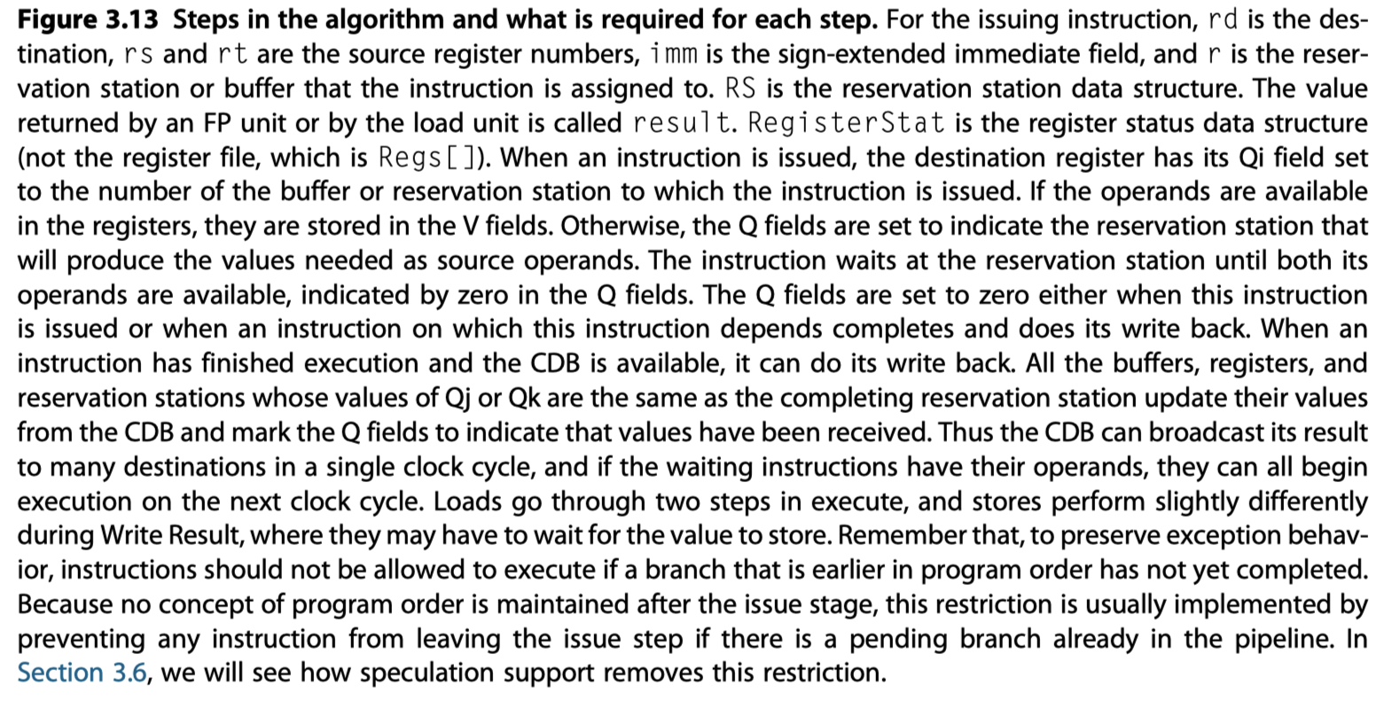
- Let’s look at the steps an instruction goes through.
- (1) Issue (or Dispatch)
- Get the next instruction from the head of the instruction queue
- No empty reservation station? $\rightarrow$ Structural hazard $\rightarrow$ Stall
- Is there a matching & empty reservation station $\rightarrow$ Issue the instruction
- How about operand values?
- Already in the registers
- $\rightarrow$ Send the operand values with the instruction to a reservation station
- Not in the registers yet?
- $\rightarrow$ Keep track of the functional units that will produce the operands
- Effectively, rename registers at this step!
- Already in the registers
- (2) Execute (or Issue)
- Not yet available operands?
- $\rightarrow$ Monitor the common data bus while waiting for it to be computed
- Become available?
- $\rightarrow$ The operation can be executed at the corresponding functional unit.
- Delaying until the operands are available
- $\rightarrow$ Avoid RAW hazard
- Multiple instructions become ready?
- $\rightarrow$ Choose arbitrarily for floating-point reservation stations, but for load/store …
-
Load/store’s two step execution process
- (1) Compute the effective address when the base register is available, then it is place in the load/store buffer
- (2) Load/store buffer execute as soon as the memory unit is available
- = So, load/store delays until both the operands (base reg) and memory unit is ready
- Preserve exception behavior
- Don’t initiate execution until a branch that precedes the instruction in program order has completed.
- i.e. The processor must know that the branch prediction was correct before allowing an instruction after the branch to begin execution
- Not yet available operands?
- (3) Write result
- When the result is available
- $\rightarrow$ Write it on the CDB
- $\rightarrow$ Into the registers
- $\rightarrow$ Into any reservation stations (including store buffers)
- When the result is available
- (1) Issue (or Dispatch)
-
Tags = Names for an extended set of virtual registers used for renaming
- Detect and eliminate hazards
- Are attached to
- the reservation stations
- the register files
- the load/store buffers
- eg. 4-bit quantity
- one of the five reservation stations or five load buffer (10 in total)
- = Equivalent of 10 registers that can be designated as result registers
- Describes which reservation station contains the instruction that will produce a result needed as a source operand
-
Forwarding and bypassing
- Implemented by …
- Common result bus $\rightarrow$ Retrieval of results by the reservation stations
- One cycle latency between source and result in a dynamically scheduled scheme
- Why? Wait until the end of the Write Result stage
-
Key difference with scoreboarding
- The tags in the Tomasulo scheme refer to the buffer or unit that will produce a result
- i.e. The register names are discarded when an instruction issues to a reservation station.
-
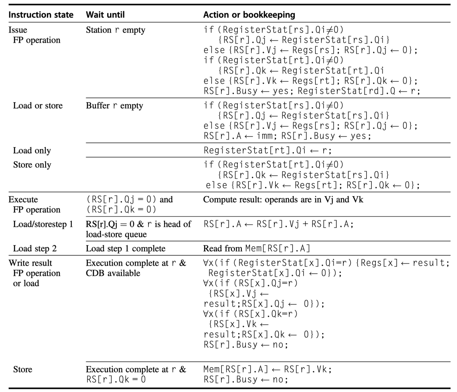
Seven fields in each reservation station
- Op (The operation to perform)
- Qj, Qk (The reservation station that will produce the corresponding source operand)
-
Vj, Vk (The value of the source operands)
- Only one of the V or Q fields is valid for each operand
- Vk = Offset field for load
- A (Information for the memory address calculation for a load or store)
- Busy (This reservation and its functional units are occupied)
-
Register file’s field
- Qi (The number (index) of the reservation station that contains the operation whose result should be stored into this register.)
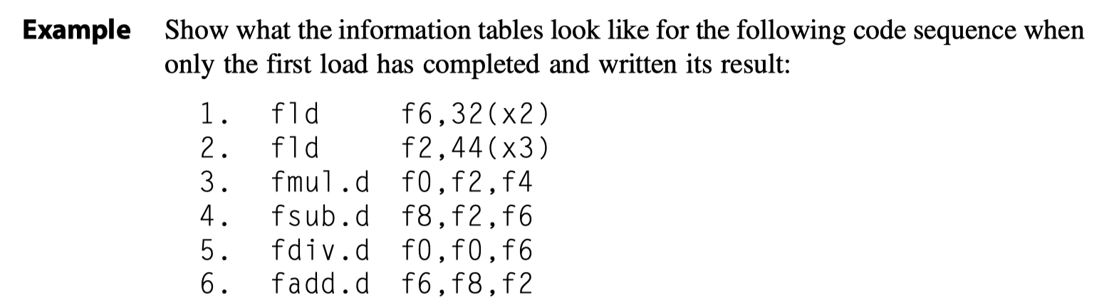
Dynamic Scheduling: Examples and the Algorithm
- Two major advantages of Tomasulo’s scheme
- (1) The distribution of the hazard detection logic
- Distributed reservation stations
- Common data bus (CDB)
- (2) the elimination of stalls for WAW and WAR hazards.
- (1) The distribution of the hazard detection logic
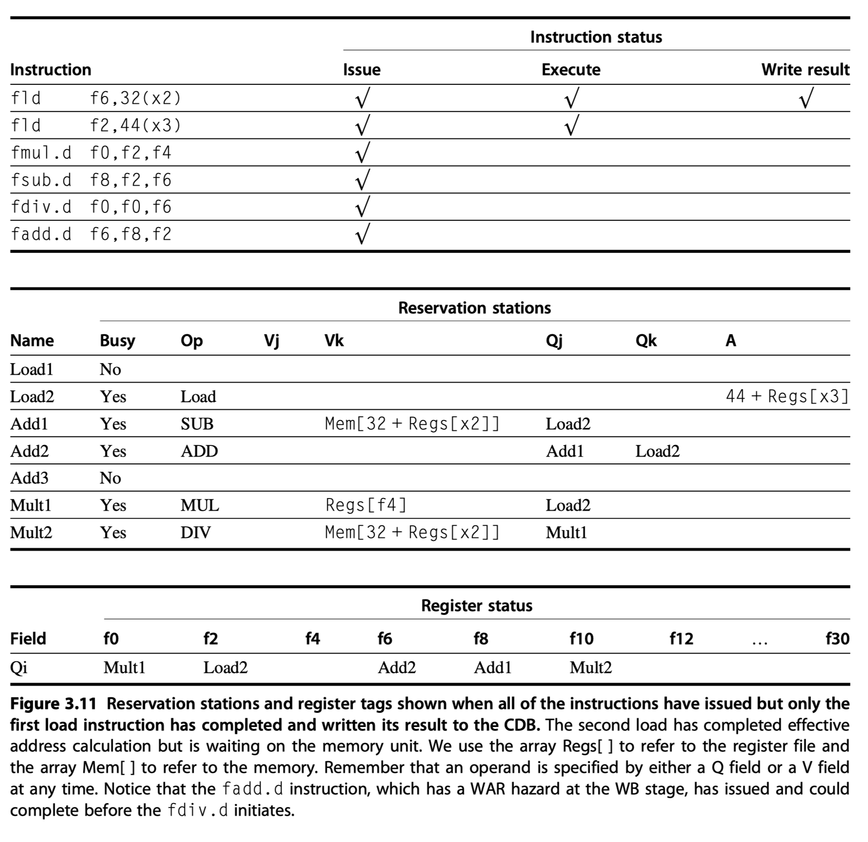
-
WAR hazard elimination in Figure 3.11
-
fdiv.dandfadd.dinvolvingf6 - Case1) If
Load1has completed $\rightarrow$Vkwill store the result $\rightarrow$fdiv.dexecutes independent offadd.d - Case2) If
Load1has not completed $\rightarrow$Qkwill point to the Load1 the result $\rightarrow$fdiv.dexecutes independent offadd.d
-
- How the example continues execution?
- Load = 1clk, Add = 2 clk, Mult = 6 clk, Div = 12 clk
- When the
fmul.dis ready to write its result …. then …

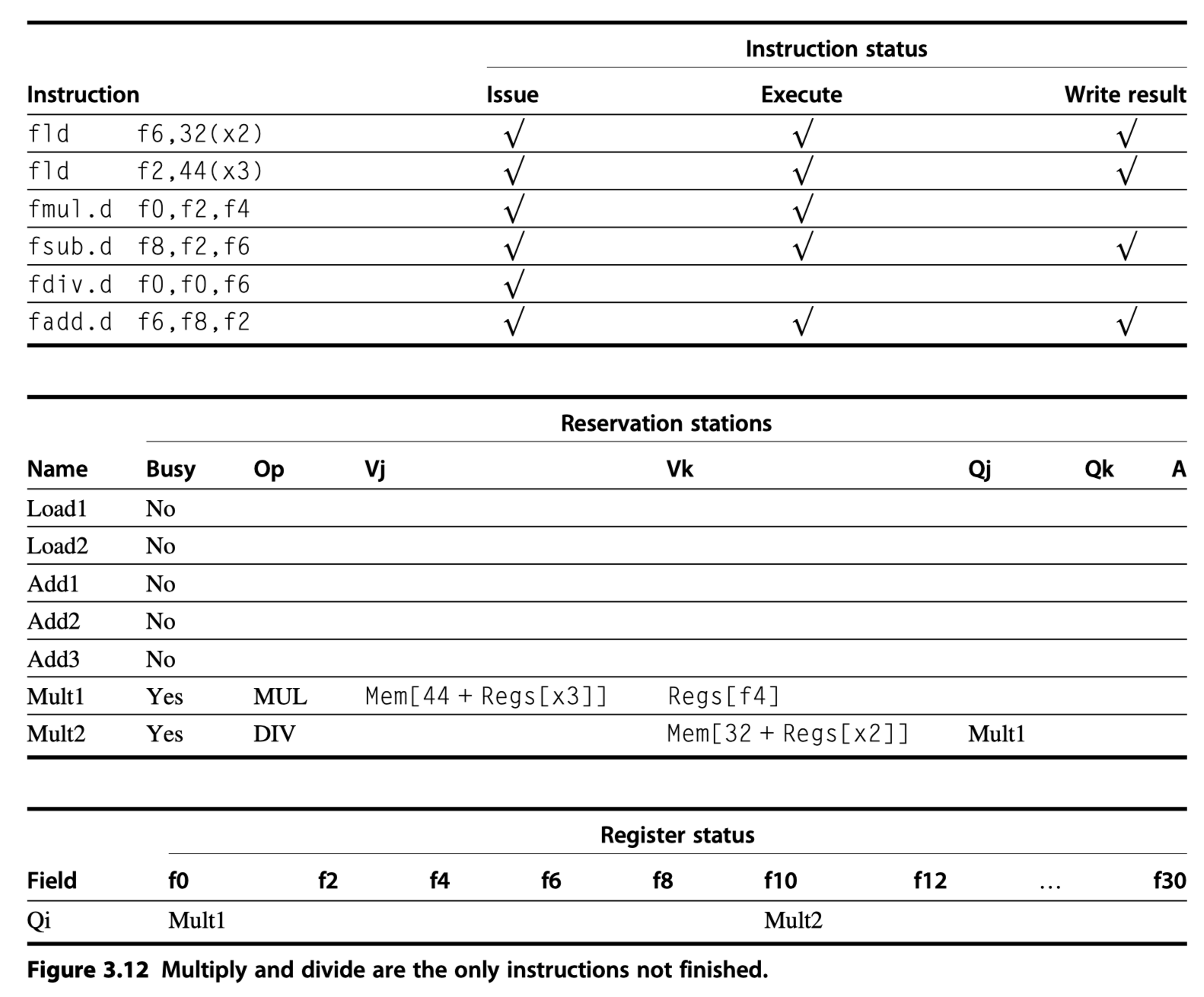
- Notice that
fadd.dis independent offdiv.d- Because the operands of
fdiv.dwere already copied - Thereby overcoming the WAR hazard
- Because the operands of
Tomasulo’s Algorithm: The Details
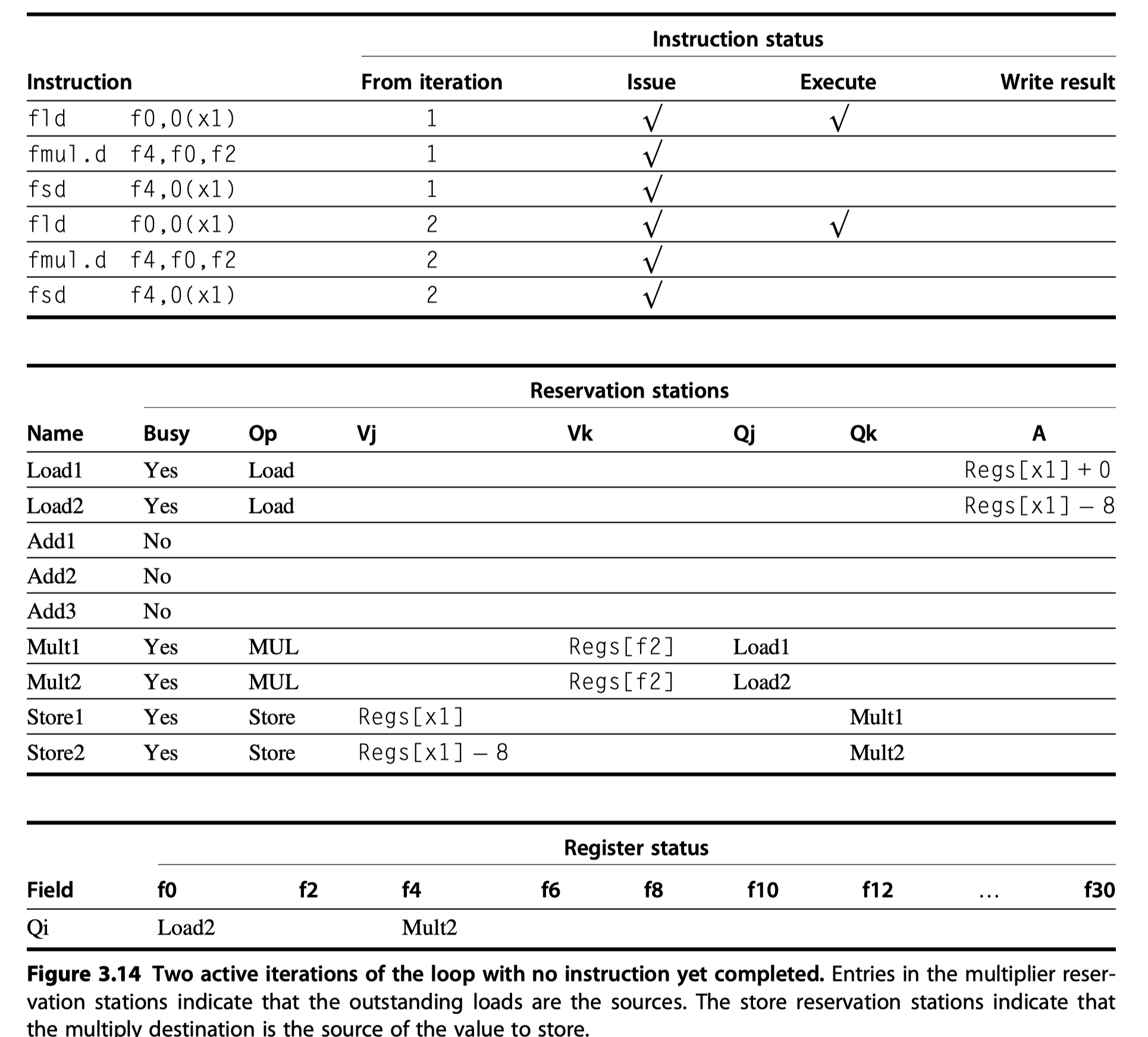
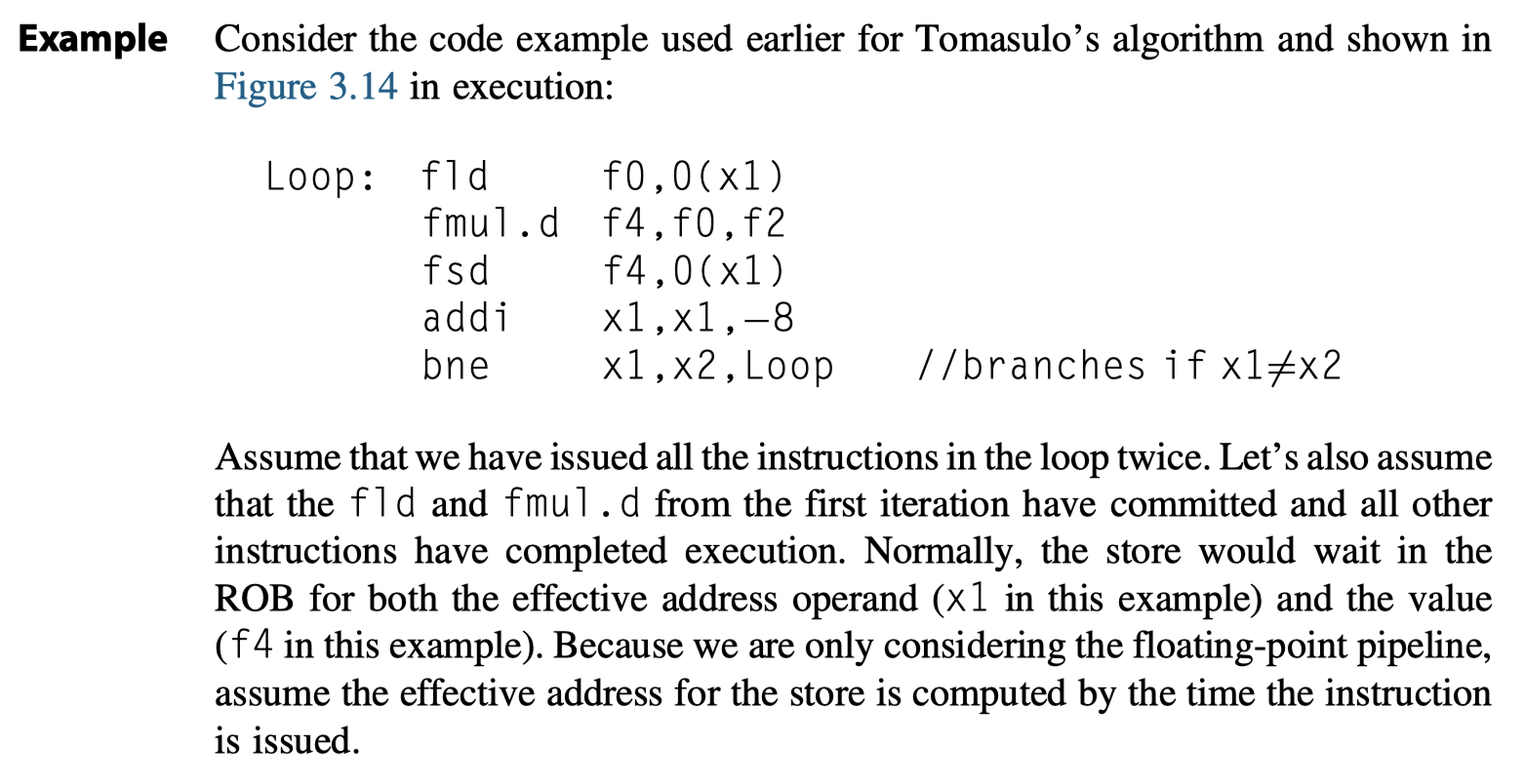
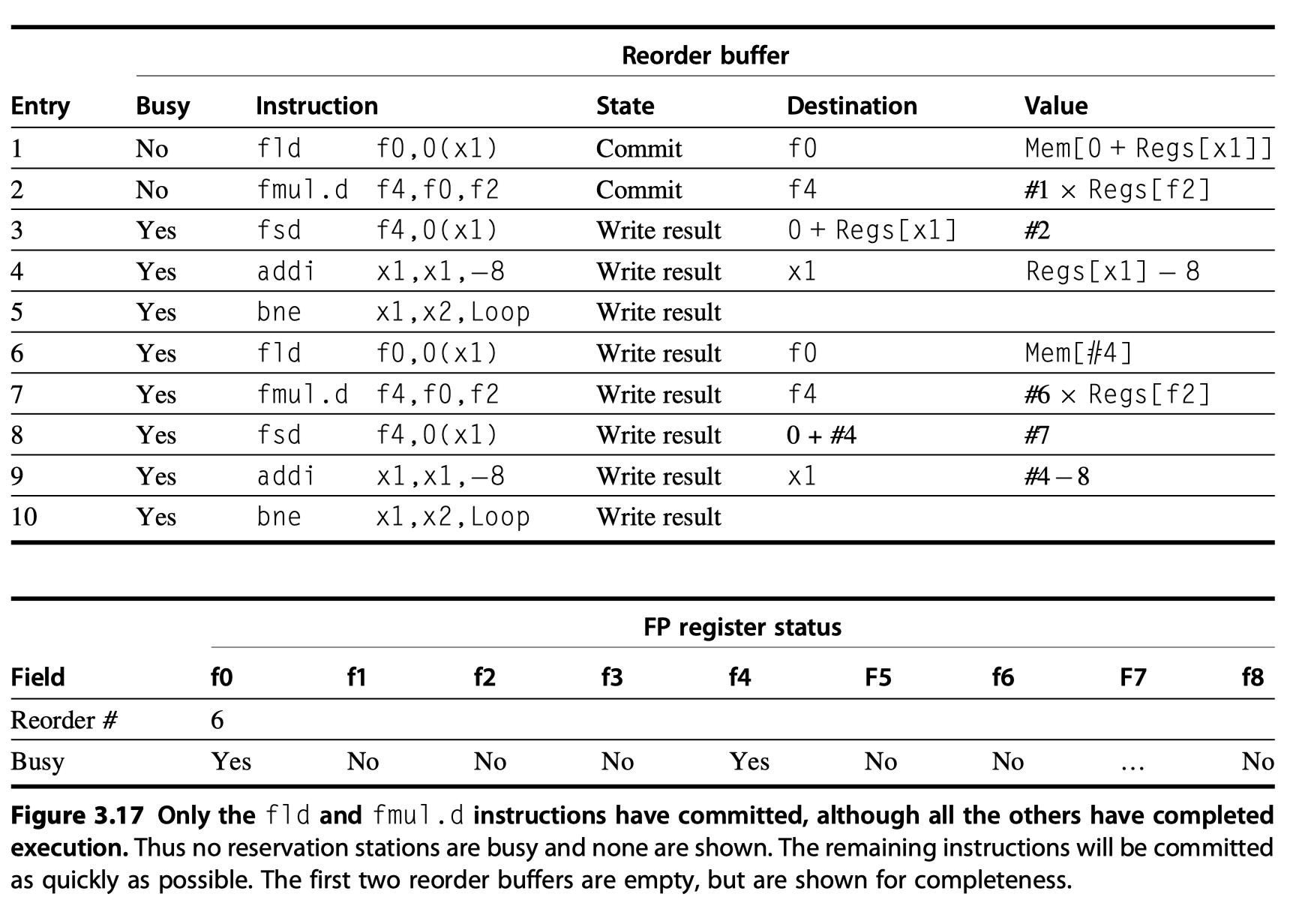
Tomasulo’s Algorithm: A Loop-Based Example
- Must look at a loop
- The full power of eliminating WAW and WAR hazards through dynamic renaming of registers
Loop:   fld f0,0(x1)
		fmul.d f4,f0,f2
		fsd f4,0(x1)
		addi x1,x1,-8
		bne x1,x2,Loop // branches if x1!=x2
- In effect, the loop is unrolled dynamically by the hardware
- using the reservation stations
- obtained by renaming to act as additional registers.
- Assume that
- we have issued all the instructions in two successive iterations of the loop,
- but none of the floating-point load/stores or operations have completed.
- At the steady state, ~1.0 CPI if the multiplies = 4 cycles
-
A load and a store
- Safely out of order, provided they access different addresses.
- Access the same address?
- (Case1) Load comes first $\rightarrow$ Interchanging $\rightarrow$ WAR hazard
- (Case2) Store comes first $\rightarrow$ Interchanging $\rightarrow$ RAW hazard
-
A store vs another store?
- (Case3) Interchanging $\rightarrow$ WAW hazard
- For execution of ….
- Load $\rightarrow$ Wait until the completion of any store that precedes the load in program order and shares the same data memory address. (RAW)
- Store $\rightarrow$ Wait until the completion of any loads and stores that precede the store in program order and shares the same data memory address. (WAR and WAW)
- So, the processors must have computed the addresses associated with any earlier memory operation.
- How? $\rightarrow$ Perform the effective address calculations in program order,
- Then, examine the A fields (a tag field with the memory address calculation for a load or store) of all active load/store buffers
- The major drawback?
- The complexity of the Tomasulo scheme
-
Large hardware overhead
- Associative tag-matching buffer
- Complex control logic
- Performance limited by single CDB
Hardware-Based Speculation
- More instruction-level parallelism?
- Overcome the limitation of control dependence!
-
Just predicting branches accurately may not be sufficient
- Speculate on the outcome of branches and execute the program as if our guesses are correct.
- Extension over branch prediction with dynamic scheduling
- We fetch, issue, and execute instructions, as if our branch predictions are always correct
- Need to handle incorrect prediction
- Speculation by
- Compiler : Appendix H
- Hardware: This section
- Three key ideas in hardware-based speculation
- (1) Dynamic branch prediction
- (2) Speculation
- Allow the execution before the control dependences are resolved
- With the ability to undo the incorrectly speculated sequence
- (3) Dynamic scheduling
- Previously, without speculation, dynamic scheduling required that a branch be resolved before execution
- Hardware-based speculation $\in$ Data flow execution!
- Operations execute as soon as their operands are available.
- How to extend Tomasulo’s algorithm?
- Separate the bypassing of results among instructions from the actual completion of an instruction
- Then, we can allow an instruction
- To execute and
- To bypass its results to other instructions
- Without allowing the instruction to perform any updates that cannot be undone, until we know that the instruction is no longer speculative.
-
Instruction commit
- An additional step in the instruction execution sequence
- When an instruction is no longer speculative,
- We allow it to update the register file or memory
- Key idea behind implementing speculation?
- Allow instructions to execute out of order but to force them to commit in order and to prevent any irrevocable action (such as updating state or taking an exception)
-
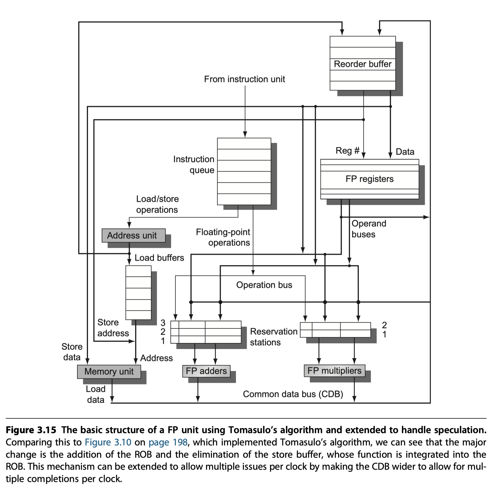
Reorder buffer (ROB)
- An additional set of hardware buffers to add the commit phase
- Hold the results of instructions that
- Have finished execution
- But have not committed
-
ROB vs Reservation stations?
- Similarity
- Provides additional registers like the reservation stations in Tomasulo’s algorithm
- So, ROB = a source of operands for instructions
- RoB ~ The store buffer in Tomasulo’s algorithm & we integrate the function of the store buffer into the ROB for simplicity
- Difference
- In Tomasulo’s algorithm, once an instruction writes its result, all subsequently issued instructions will find the result in the register file.
- With speculation, the register file is not updated until the instruction commits
- Similarity
- So, the ROB supplies operands in the interval between completion of instruction execution and instruction commit.
- Four fields in each entry in the ROB
-
Instruction type
- a branch?
- a store?
- a register operation?
-
Destination field
- Register number
- Memory address
-
Value field
- Hold the values until the instruction commit
-
Ready field
- Completed execution and waiting for commit
-
Instruction type
-
Store buffers included in ROB
- Two steps (address + memory-ready)
- The second step (memory-ready) is performed by instruction commit
- Renaming function of the reservation stations is replaced by the ROB
- Two steps (address + memory-ready)
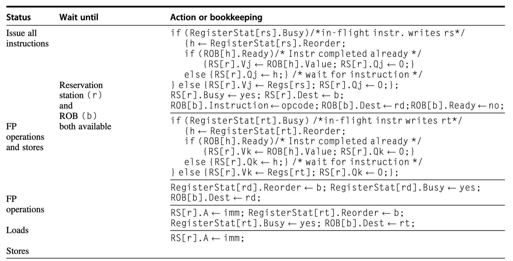
- Four steps involved in instruction execution
-
(1) Issue
- Get an instruction from the instruction queue
- Issue if there is
- an empty reservation station and
- an empty slot in the ROB
- i.e. Check structural hazard
- Send ..
- Instruction (with available operands and ROB entry number) to a reservation station
-
(2) Execute
- Monitor CDB if any operand is not available yet (So, check RAW hazard)
- Execute if all operands are ready in the reservation station
-
(3) Write result
- Result ready?
- $\rightarrow$ Write it on the CDB
- $\rightarrow$ ROB and reservations waiting for the results
- With ROB tag sent when the instruction issued
-
(4) Commit (a.k.a., “completion” or “graduation”)
- Only results remains here
-
(Case1) Normal commit case
- Instruction reaches the head of the ROB
- Its result is present in the buffer
- Updates the register (memory for store) with the results
- Remove the instruction from the ROB
-
(Case2) Correct speculation
- The branch is finished
-
(Case3) Wrong speculation
- A branch with incorrect prediction reaches the head of the ROB
- ROB is flushed
- Execution is restarted at the correct successor of the branch
-
(1) Issue
- The same example we used for Tomasulo’s algorithm.
- 2 cycle for
add, 6 cycles formult, 12 cycles fordivexecution
- 2 cycle for
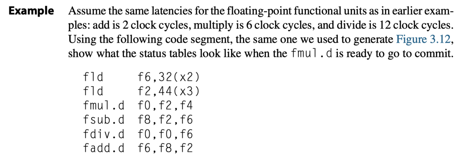
- When
fmul.dis ready to commit …
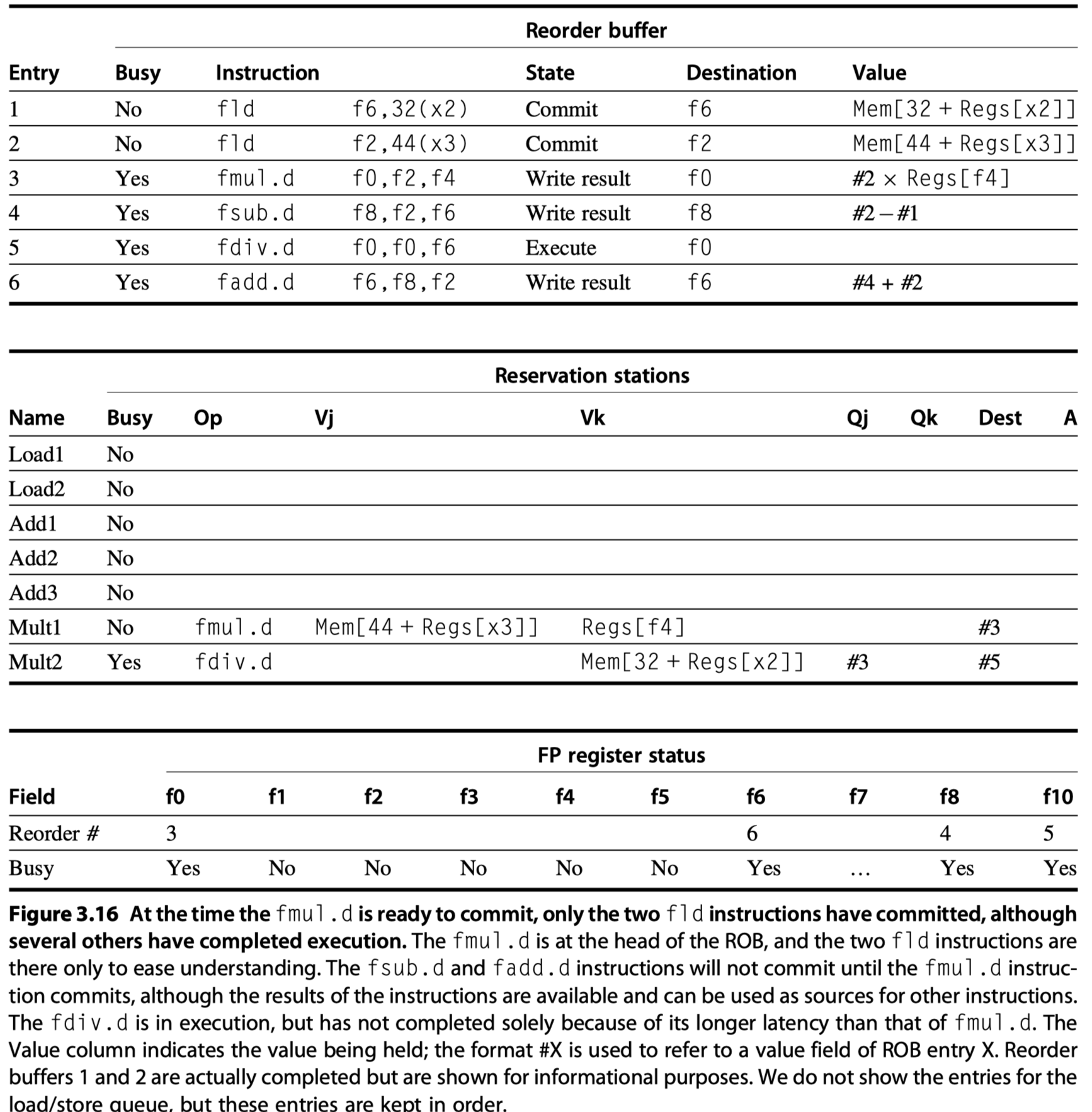
- The differences in tags between Tomasulo’s algorithm without and with speculation are that
- (1) reservation station numbers are replaced with ROB entry numbers in the Qj and Qk fields, as well as
- (2) in the register status fields, and we added the Dest field to the reservation stations. The Dest field designates the ROB entry that is the destination for the result produced by this reservation station entry
- Key difference in performance between Tomasulo’s algorithm without and with speculation ?
- Without speculation, no instruction after the earliest uncompleted instruction (
fmul.din preceding example) is allowed to complete - With speculation, later instructions (
fsub.dandfadd.d) instructions have also completed. - Why?
- The processor with the ROB can dynamically execute code while maintaining a precise interrupt model.
- If
fmul.dcauses interrupt?- Simply flush any other pending instructions (
fsub.dandfadd.d) from ROB! - Without ROB,
fsub.dandfadd.dcan overwritef8andf6$\rightarrow$ Imprecise exception!!
- Simply flush any other pending instructions (
- Without speculation, no instruction after the earliest uncompleted instruction (
- The use of a ROB with in-order instruction commit provides precise exceptions
- If the first branch is mispredicted,
- Instructions prior to the branch $\rightarrow$ Simply commit when each reaches the head of the ROB
- Mispredicted branch reaches the head of the buffer $\rightarrow$ Simply clear the buffer!
- Exception
- If a speculated instruction raises an exception
- Record the exception in the ROB
- Mispredicted $\rightarrow$ The exception is flushed
- Correctly predicted $\rightarrow$ Take the exception
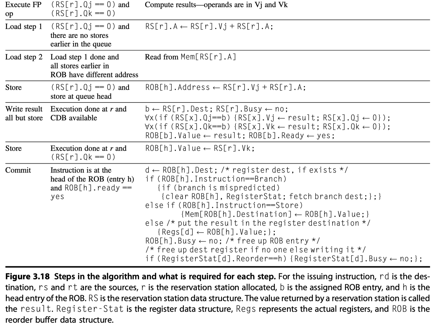
- Figure 3.18 shows the steps of execution for an instruction
- Compare Figure 3.18 vs Figure 3.13 (without speculation)
- Speculation adds significant complications to the control
- Branch mispredictions are somewhat more complex.
Exploiting ILP Using Multiple Issue and Static Scheduling
-
Improve performance further?
-
Multiple-issue processors!
-
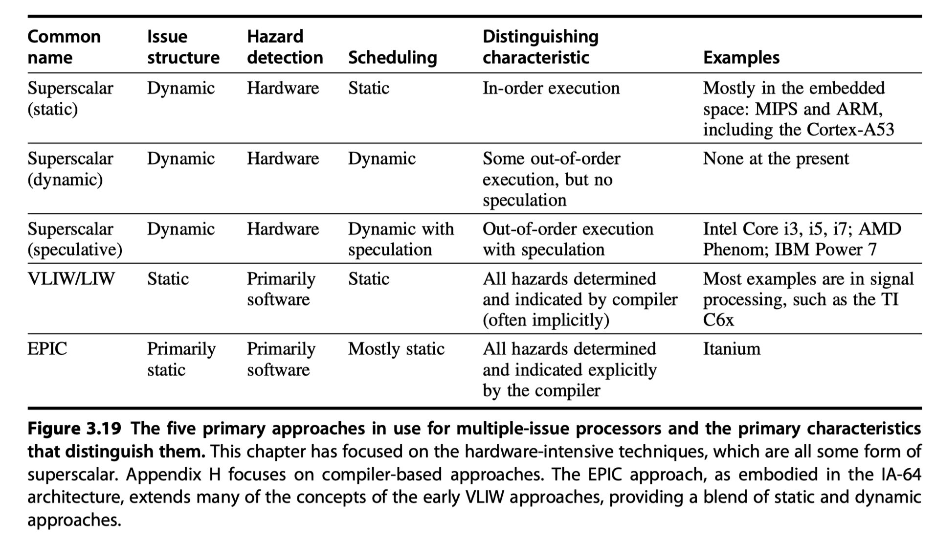
Statically scheduled superscalar processors
- Varying numbers of instructions per clock and use in-order execution
- Rely on the compiler
- Closer to VLIWs
- Diminishing advantage as the issue width grows $\rightarrow$ Normally used for just two instruction width
-
VLIW (very long instruction word) processors
- Fixed number of instructions
- Formatted either as
- One large instruction
- A fixed instruction packet with instruction parallelism
- Inherently statically scheduled by the compiler
-
Dynamically scheduled superscalar processors
- Varying numbers of instructions per clock and use out-of-order execution
-
Statically scheduled superscalar processors
Basic VLIW Approach
-
Uses multiple, independent functional units
-
VLIW packages the multiple operations into one very long instruction
- Let’s consider VLIW with instructions with five operations
- One integer
- Two floating-point
- Two memory references
- A set of fields in an instruction for each functional units
- 16-24 bits per unit
- 80-120 bits per instruction
- eg. Intel Itanium1/2 = Six operations per instruction packet + concurrent issue of two/three instruction bundle
- Enough parallelism in a code sequence
- To keep the functional units busy
- Unrolling loops and scheduling the code within the single larger loop body
- Parallelism in a straight-line code? $\rightarrow$ Local scheduling
- Parallelism across branches? $\rightarrow$ Global scheduling (more complex)

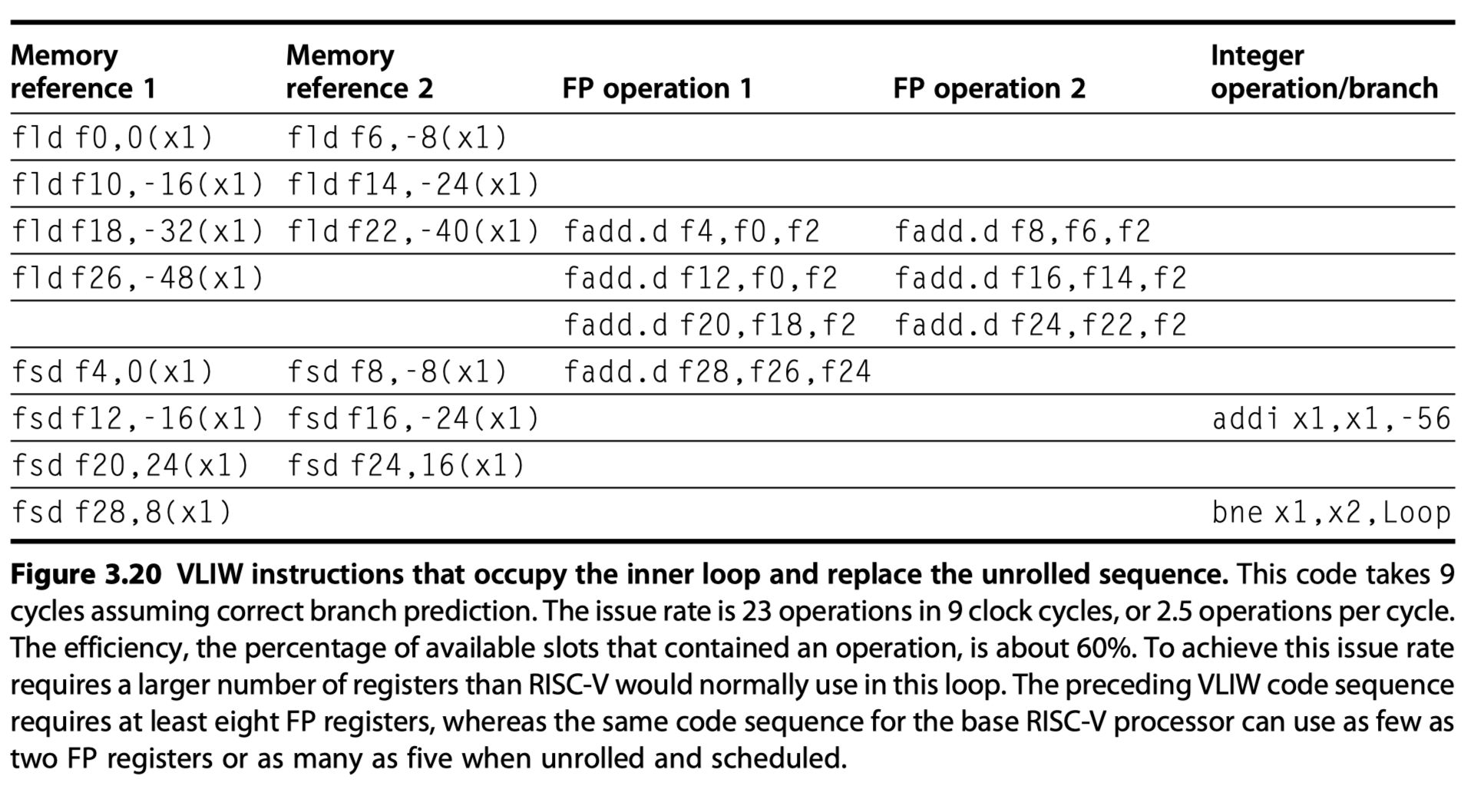
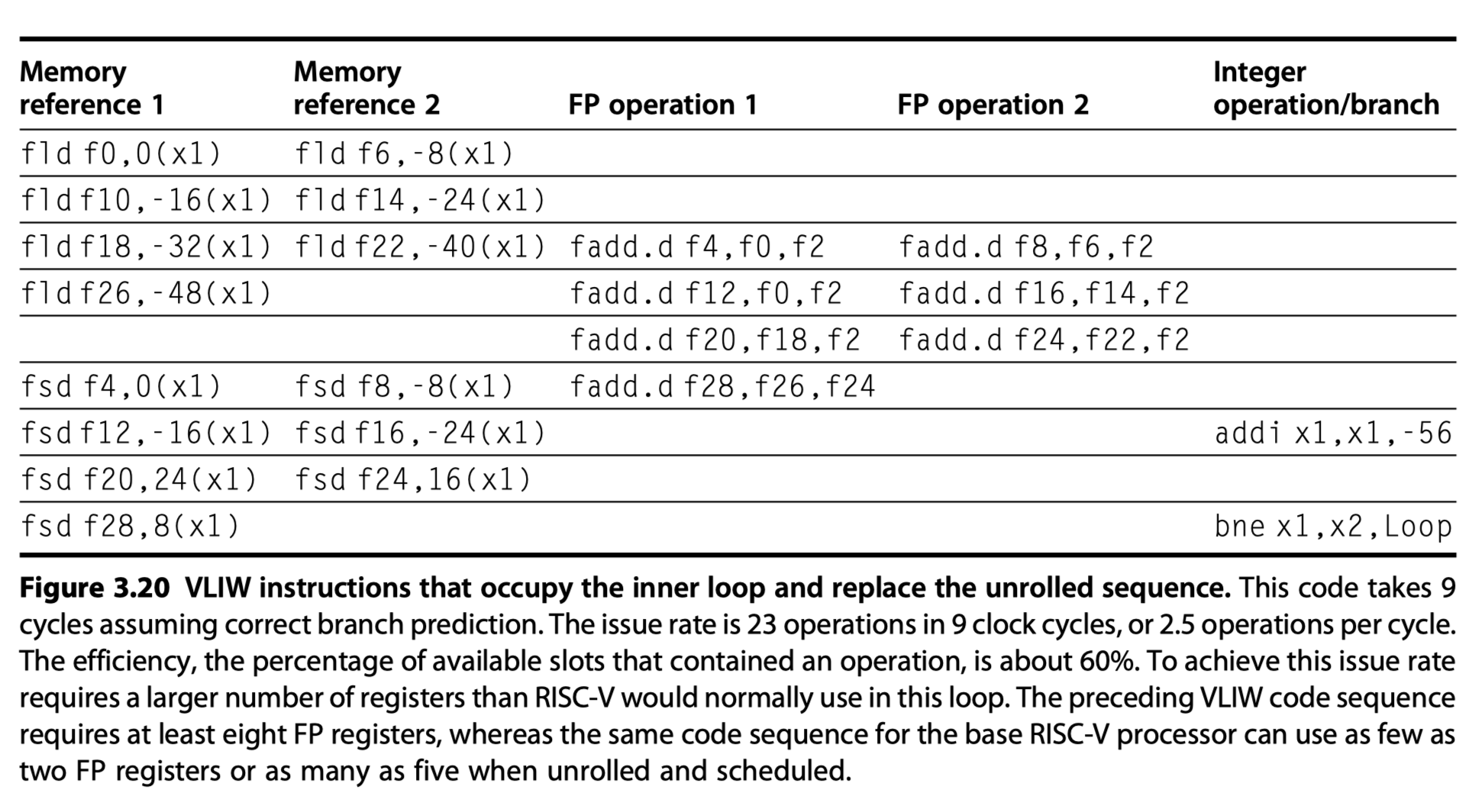
- VLIW for loops
- Two memory references, two FP operations, and one integer operation in an instruction
- Loop unrolling
- Seven copies of the body
- 23 Operations
- Run in 9 cycles
- 2.5 operations per cycle
- 1.29 cycle per result
-
Original VLIW model’s problems
- Large code size $\rightarrow$ Need clever encodings
- Limitation of the lockstep operation
- Early VLIW operated in lockstep without hazard-detection hardware
- All functional units had to be synchronized
- So, stall in any functional unit $\rightarrow$ Need to stall the entire processor
- Caches $\rightarrow$ Blocking, causing all the functional units to stall
- Larger issue rate $\rightarrow$ Unacceptable synchronization restriction
- Binary code compatibility
- Different number of functional units $\rightarrow$ Different versions of the code
-
Multiple-issue processors vs Vector processors?
- Multiple-issue :
- Loops $\rightarrow$ Need unrolling
- Good to extract ILP for less structured codes
- Easily cache all forms of data
- So, primary method for ILP
- Vector :
- Loops $\rightarrow$ Original code is good enough $\rightarrow$ More simple and efficient
- So, extension to multiple-issu processors
- Multiple-issue :
Exploiting ILP Using Dynamic Scheduling, Multiple Issue, and Speculation
- Put all (1) dynamic scheduling, (2) multiple issue, and (3) speculation together!
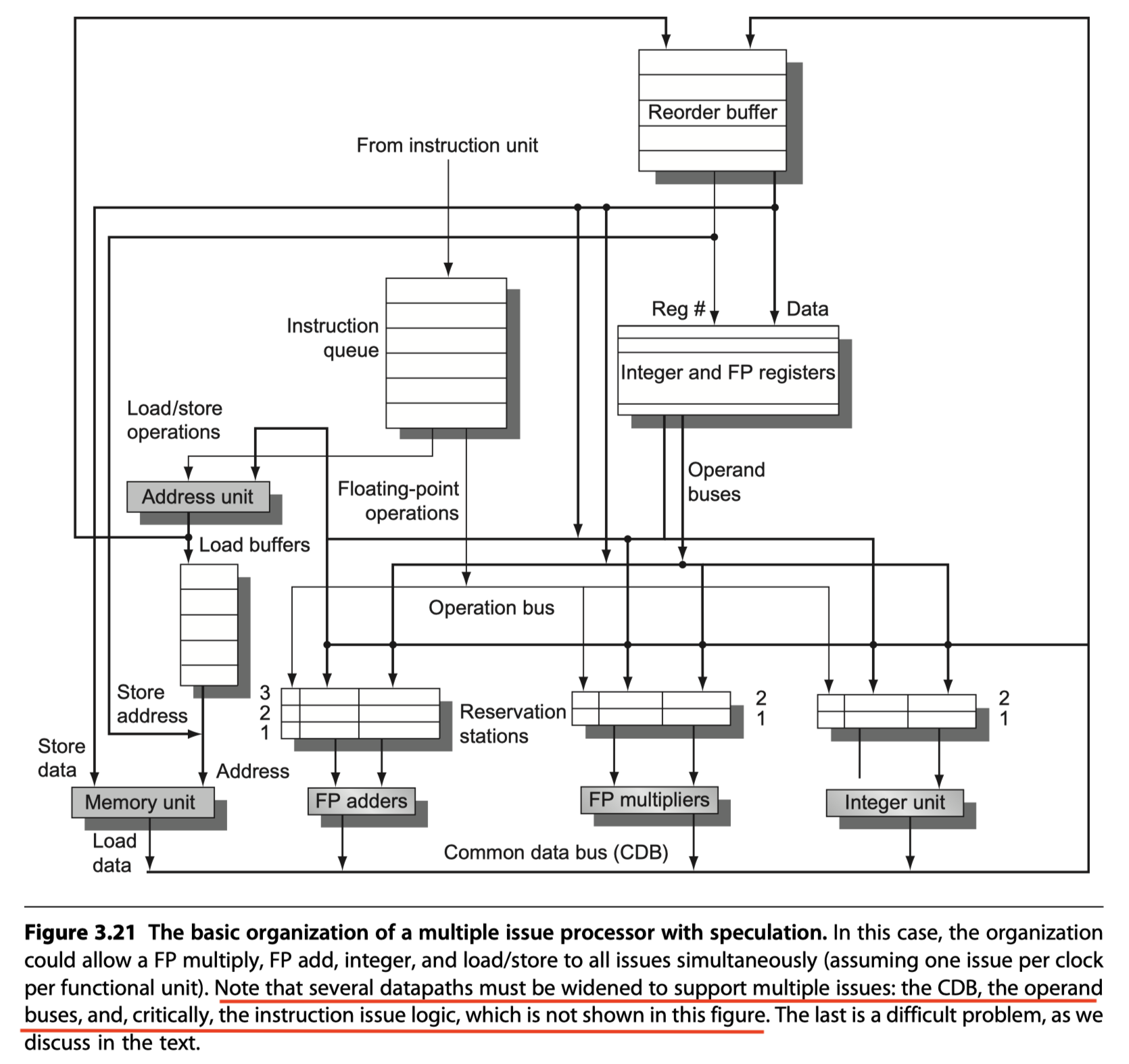
- $\rightarrow$ Microarchitectures in modern microprocessors
- The basic organization of a multiple issue processor with speculation
- Tomasulo’s algorithm
- Multiple issue superscalar pipeline
- Issue rate of two instructions per clock
- Using the scheduling hardware
- Separate integer
- Load/Store
- Floating-point units (FP multiply and FP add)
- Don’t issue instructions to the reservation stations out of order
- To avoid violation of program semantics
- Complexity of multiple instruction issuing
- Multiple instructions may depend on one another $\rightarrow$ The tables must be updated for the instructions in parallel
- (Todo#1) Assign a reservation station
- (Todo#2) Update the pipeline control tables
- (Approach#1 : Pipeline the issue logic) Run this step in half a clock cycle $\rightarrow$ Two instructions can be processed in one clock cycle $\rightarrow$ Not scalable for four instructions
- (Approach#2 : Widen the issue logic) Build the logic necessary to handle two or more instructions at once, including any possible dependences between the instructions
- Modern superscalar processors includes both approaches
- Issue logic example (Figure 3.22)
- Most fundamental bottlenecks in dynamically scheduled superscalars
- Every possible combination of dependent instructions $\varpropto$ (#instructions issued in a cycle)$^2$
- Issuing a load followed by a dependent FP operation
- Based on that in Figure 3.18
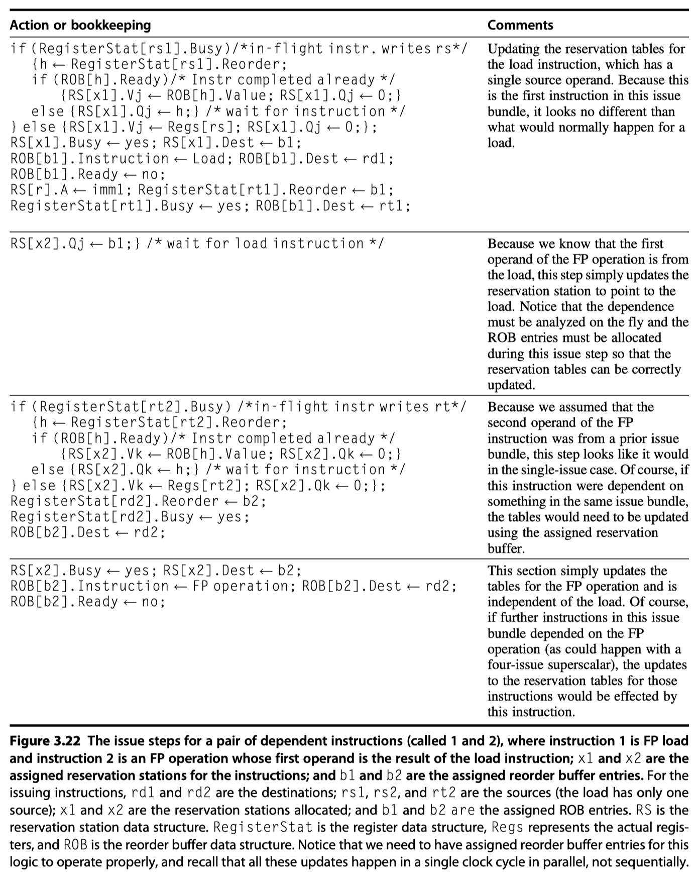
- Most fundamental bottlenecks in dynamically scheduled superscalars
- Generalized issue logic in a dynamically scheduled superscalar processor
- Assign (Preallocate) a reservation station and a reorder buffer for every instruction that might be issued in the next issue bundle.
- Without knowing the instruction types
- By limiting #instructions of a given class (eg. one FP, one integer, one load, one store)
- If not sufficient reservation station? $\rightarrow$ Break the bundle $\rightarrow$ Issue in two or more cycles
- Analyze all the dependences among the instructions in the issue bundle.
- If an instruction in the bundle depends on an earlier instruction in the bundle, use the assigned reorder buffer number to update the reservation table for the dependent instruction.
- Do all the steps in one cycle !!
- Assign (Preallocate) a reservation station and a reorder buffer for every instruction that might be issued in the next issue bundle.
- Back-end of the pipeline
- Complete and commit multiple instructions per clock
- Easier than the issue problems due to already resolved dependence
- Intel i7 in Section 3.12
- Speculative multiple issue
- A large number of reservation stations
- A reorder buffer
- A load and store buffer
- Also used to handle nonblocking cache misses
-
Loop with a two-issue processor

- Without speculation
- Execution of
ldshould wait untilbneis executed - Third branch $\rightarrow$ clock cycle 19
- Execution of
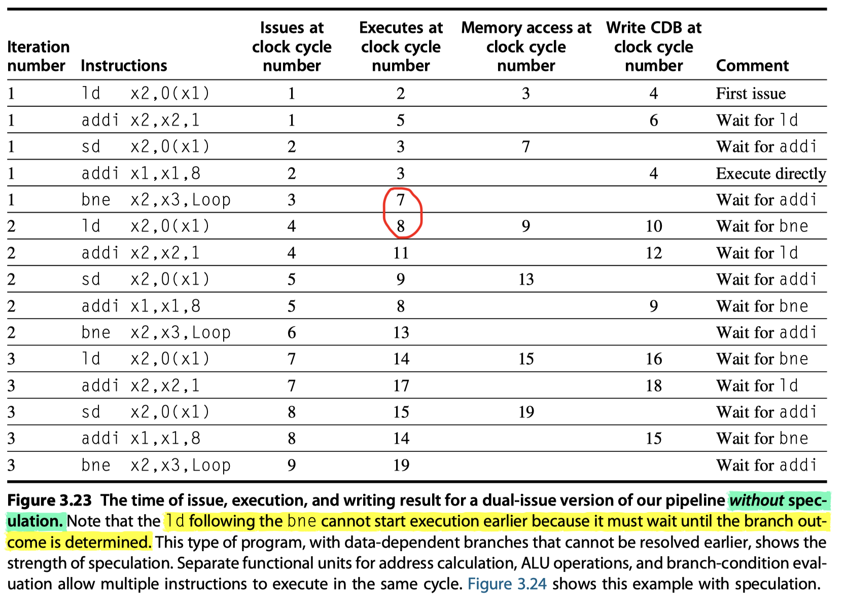
- With speculation (+ Correct prediction)
-
ldcan be executed before we knowbneresult with speculation !! - Commit of
ldinstruction happen after that ofbneinstruction - Third branch $\rightarrow$ clock cycle 13
-

Advanced Techniques for Instruction Delivery and Speculation
- Advanced-Techniques
- (1) Have to be able to deliver a high-bandwidth instruction stream
- 4-8 instructions every clock cycle
- (2) Use of register renaming versus reorder buffers
- (3) The aggressiveness of speculation
- (4) Value prediction
- (1) Have to be able to deliver a high-bandwidth instruction stream
Increasing Instruction Fetch Bandwidth
- High instruction bandwidth?
- Widen paths to the i$
- Difficult part? = Handling branches !!
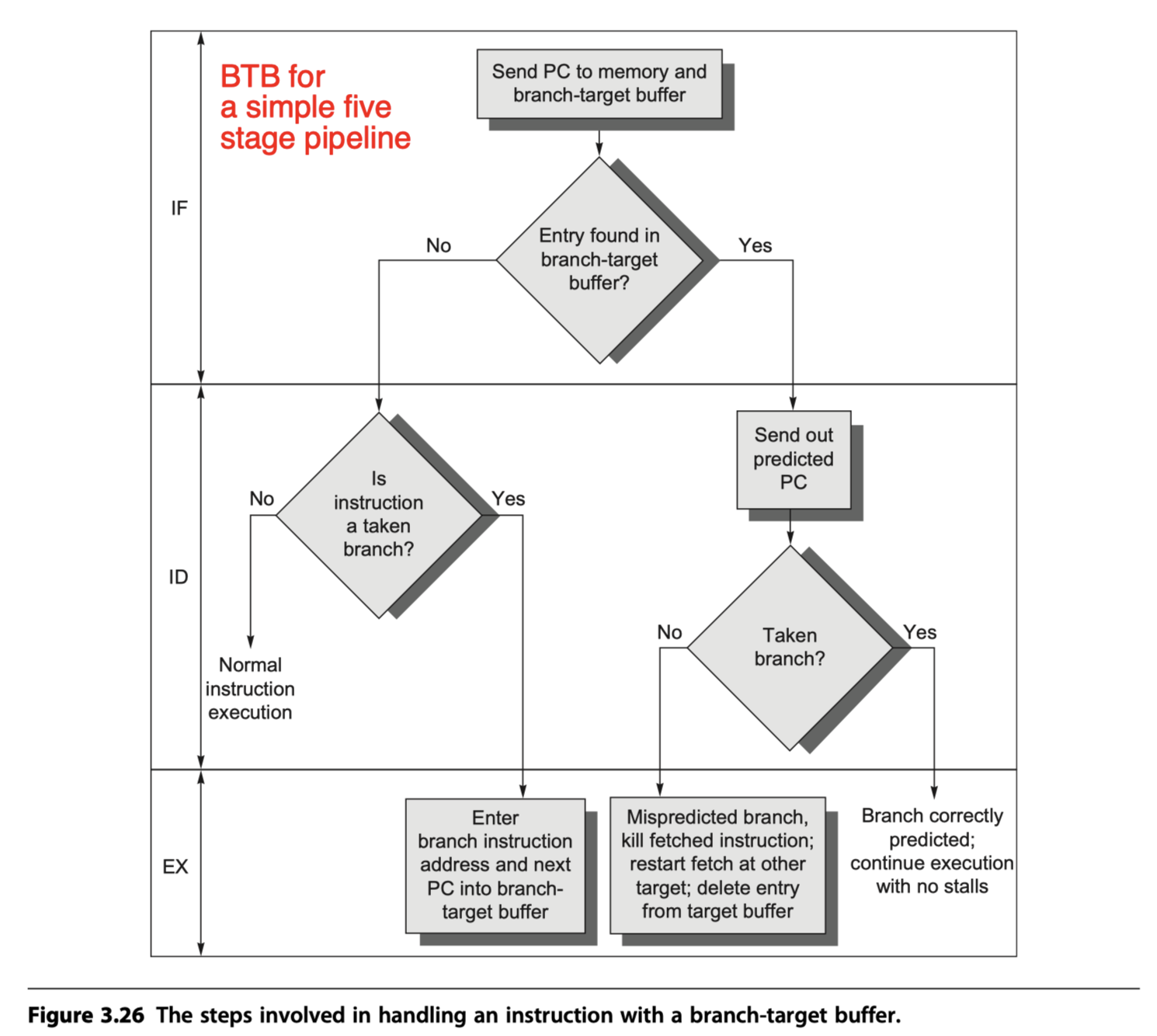
Branch-Target Buffers
- Reduce the branch penalty?
- Must know whether the as-yet-undecoded instruction is a branch and, if so, what the next program counter (PC) should be.
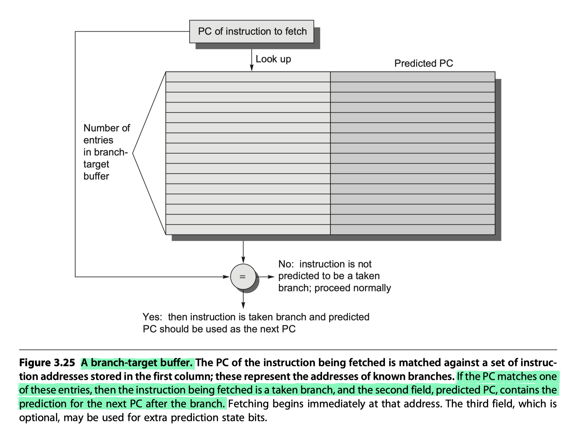
- Branch-target buffer
- or Branch-target cache
- A branch-prediction cache that stores the predicted address for the next instruction after a branch
- A BTB predicts the next instruction address and will send it out before decoding the instruction
- Cache-like steps in BTB
- (1) If the PC of the fetched instruction matches an address (at the first column in Figure 3.25) in the prediction buffer,
- It means that the branch instruction is predicted as a taken branch !!
- (2) then the corresponding predicted PC (at the second column in Figure 3.25) is used as the next PC.
- i.e. If a matching entry is found in the branch-target buffer, fetching begins immediately at the predicted PC.
- Same with tag-matching steps in hardware caches
- Note that unlike a branch-prediction buffer (False branch-prediction buffer only reduce prediction accuracy), the predictive entry must be matched to this instruction (if not, possible to fetch completely wrong instructions)
- (1) If the PC of the fetched instruction matches an address (at the first column in Figure 3.25) in the prediction buffer,
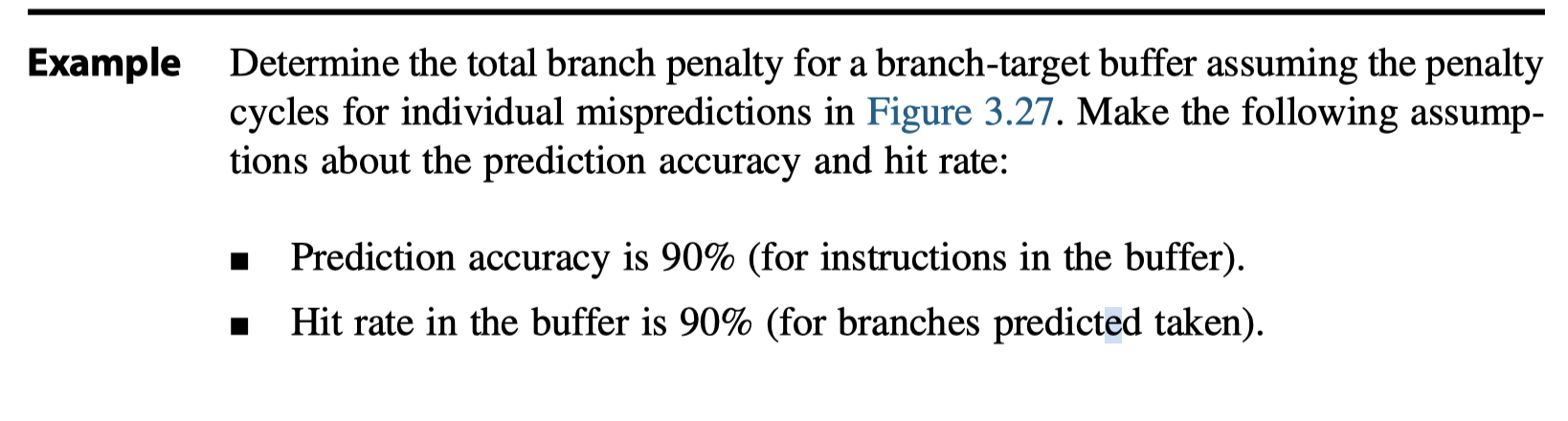
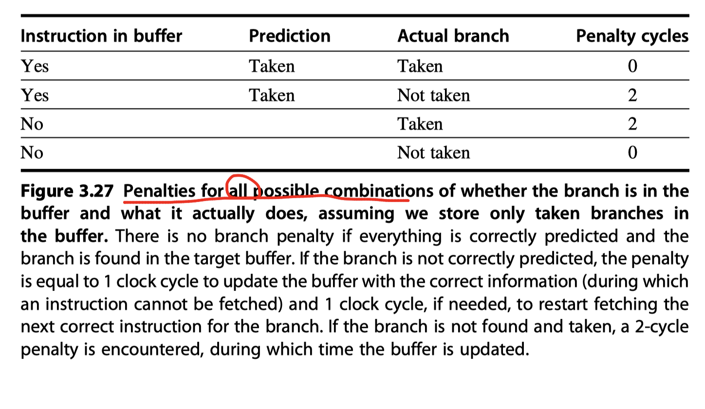
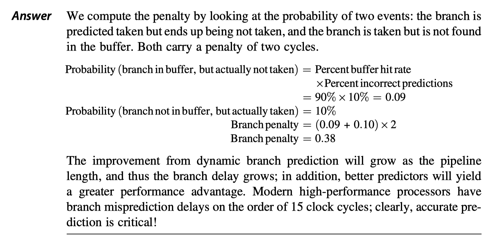
- No branch delay if a branch-prediction entry is found in the buffer and the prediction is correct.
- Otherwise, penalty at least 2 cycles
- Otherwise, penalty at least 2 cycles
- Variation: Store target instructions instead of (or in addition to) target addresses
- (Advantage#1) Allow longer time $\rightarrow$ Allow larger BTB
- (Advantage#2) Allow optimization called branch folding
- Obtain 0-cycle unconditional branches and sometimes 0-cycle conditional branches.
Specialized Branch Predictors: Predicting Procedure Returns, Indirect Jumps, and Loop Branches
-
Challenge of predicting indirect jumps whose destination address varies at runtime
-
Indirect jumpfrom chatGPT:- In C++, an indirect jump instruction occurs when a function pointer is used to jump to a function at runtime.
- In C++, function pointers are variables that hold the address of a function. They can be assigned to, passed as arguments to other functions, and returned from functions. When a function pointer is dereferenced (using the
*operator), it is treated as a function call. - Here’s an example of how an indirect jump can occur in C++ code using a function pointer
- In this example,
pis a function pointer that holds the address offoo. The expression(*p)()dereferencespand callsfooindirectly. This is an example of an indirect jump because the specific function being called (= procedure being returned) is determined at runtime based on the value ofp.
1
2
3
4
5
6
7
8
9
10
11


#include <iostream>

void foo() {
	std::cout << "Hello, world!\n";
}
int main() {
	void (*p)() = &foo; // p holds the address of foo
	(*p)(); // dereference p and call foo
	return 0;
}
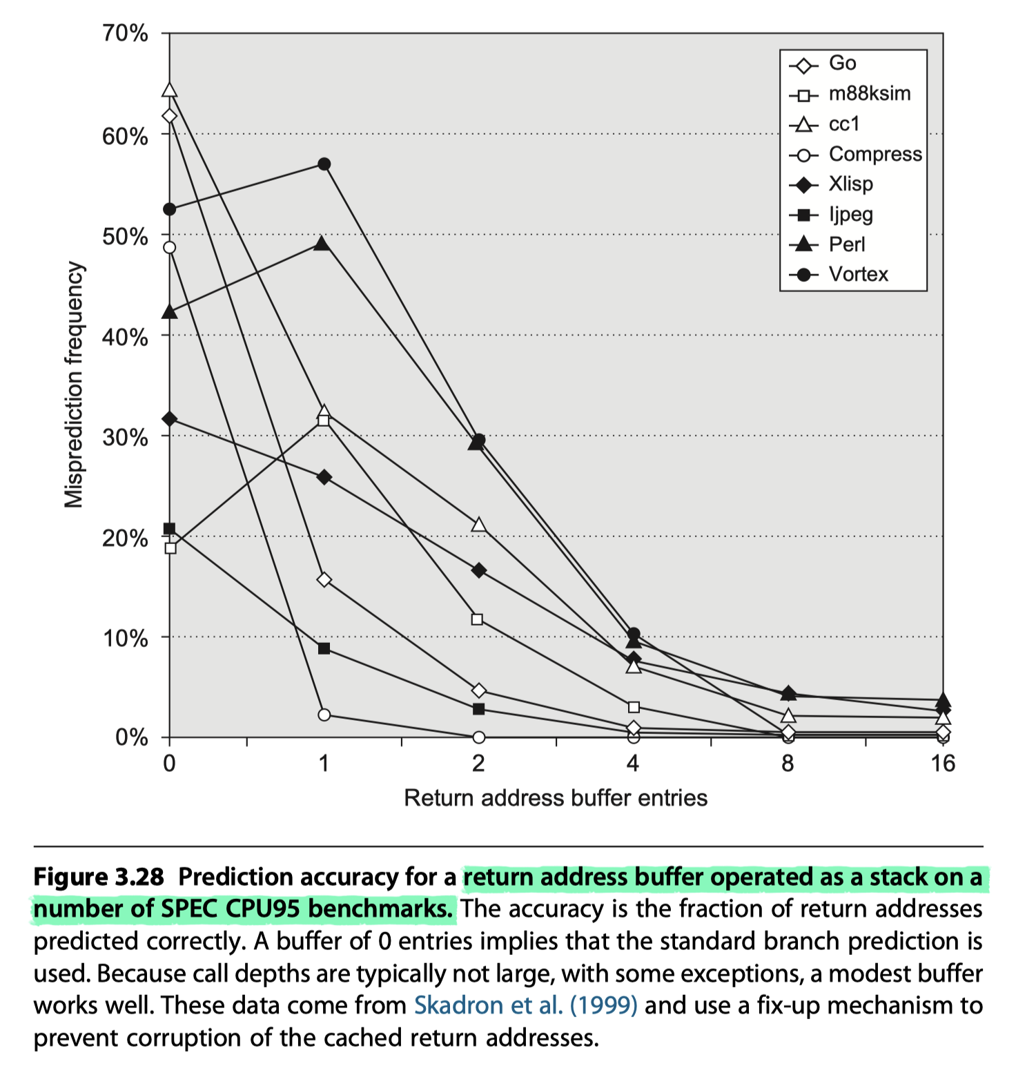
- Procedure returns (like function pointer)
- Can be predicted with a branch-target buffer with low the accuracy
- If the procedure is called from multiple sites with low spatial/temporal locality
- To overcome this problem,
- Some designs use a small buffer of return addresses operating as a stack. (Return address buffer or Return address stack, RAS)
- (1) Cache the most recent return addresses,
- (2) Pushing a return address on the stack at a call and popping one off at a return.
- Some designs use a small buffer of return addresses operating as a stack. (Return address buffer or Return address stack, RAS)
Integrated Instruction Fetch Units
- A separate autonomous unit that feeds instructions to the rest of the pipeline
- Integrated branch prediction
- Instruction prefetch (see Chapter 2 for a discussion of techniques for doing this)
- Instruction memory access and buffering
- Accessing multiple cache lines for fetching multiple instructions using prefetch to try to hide the cost of crossing cache blocks
- Also provides buffering, essentially acting as an on-demand unit to provide instructions to the issue stage as needed and in the quantity needed.
Speculation: Implementation Issues and Extensions
Speculation Support: Register Renaming Versus Reorder Buffers
- How to implement speculation on top of Tomasulo’s algorithm?
- (1) Use a reorder buffer (ROB)
- Register values may also temporarily reside in the ROB
- So, no register renaming is necessary
- (2) An alternative : Explicit register renaming
- An extended set of physical registers is used to hold both the architecturally visible registers (
x0, . . .r31andf0, . . .f31) as well as temporary values. - Thus the extended registers replace most of the function of the ROB and the reservation stations
- An extended set of physical registers is used to hold both the architecturally visible registers (
- (1) Use a reorder buffer (ROB)
-
Renaming map
- A renaming process (during instruction issue) maps …
- The names of architectural registers to physical register numbers in the extended register set,
- Allocating a new unused register for the destination.
- Advantage of explicit register renaming vs reorder buffer?
- Instruction commit is slightly simplified
- (1) Record that the mapping between an architectural register number and physical register number is no longer speculative
- (2) Free up any physical registers being used to hold the “older” value of the architectural register.
- In a design with reservation stations, a station is freed up when the instruction using it completes execution, and a ROB entry is freed up when the corresponding instruction commits.
- Instruction commit is slightly simplified
- Disadvantage?
- Deallocating registers is more complex (Must know that the physical register will not be used)
- A strategy for instruction issue with explicit register renaming similar to ROB case
- The issue logic reserves enough physical registers for the entire issue bundle
- The issue logic determines what dependences exist within the bundle.
- With dependences within the bundle: The register renaming structure is used to determine the physical register that holds, or will hold, the result on which instruction depends.
- Without dependence within the bundle: The result is from an earlier issue bundle, and the register renaming table will have the correct register number
- With dependences with the earlier bundles: The pre-reserved physical register in which the result will be placed is used to update the information for the issuing instruction.
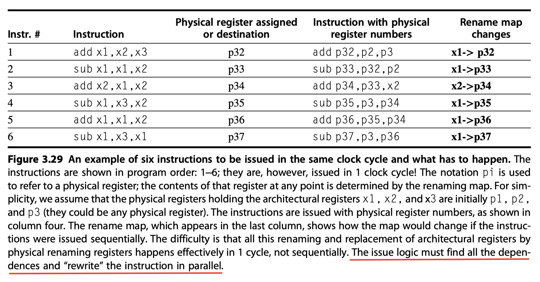
The Challenge of More Issues per Clock
- Let’s take a look at what has to happen for a six-issue processor using register renaming.
- In a single cycle !
- All the dependences must be detected
- The physical registers must be assigned
- The instructions must be rewritten using the physical register numbers
How Much to Speculate?
- To maintain most of the advantage while minimizing the disadvantages,
- Most pipelines with speculation will allow only low-cost exceptional events (such as a first-level cache miss) to be handled in speculative mode
- Don’t allow an expensive exceptional events, such as a second-level cache miss or a TLB miss
Speculating Through Multiple Branches
- Speculate on multiple branches simultaneously when …
- (Case#1) a very high branch frequency,
- (Case#2) significant clustering of branches, and
- (Case#3) long delays in functional units.
Speculation and the Challenge of Energy Efficiency
- Excess energy consumption
- Instructions that are speculated and whose results are not needed generate excess work for the processor
- Undoing the speculation and restoring the state of the processor to continue execution at the appropriate address
Address Aliasing Prediction
-
Address aliasing prediction
- A technique that predicts whether two stores or a load and a store refer to the same memory address.
- If two such references do not refer to the same address, then they may be safely interchanged.
- Otherwise, we must wait until the memory addresses accessed by the instructions are known.
-
Value prediction $\ni$ Address prediction
- Have never been sufficiently attractive
Cross-Cutting Issues
Hardware Versus Software Speculation
- To speculate extensively, we must be able to disambiguate memory references.
-
- Support for speculative memory references
-
- Hardware-based speculation works better when control flow is unpredictable than software-based approach
- Hardware-based speculation
- Maintains a completely precise exception model even for speculated instructions.
- Does not require compensation or bookkeeping code
- Does not require different code sequences
- The major disadvantage of supporting speculation in hardware is the complexity and additional hardware resources required.
Speculative Execution and the Memory System
- The possibility of generating invalid addresses with speculation is inherent
- Incorrect behavior if protection exceptions were taken
- Swamped by false exception overhead
- So, the memory system must
- identify
- speculatively executed instructions and
- conditionally executed instructions
- suppress the corresponding exception.
- not allow such instructions to cause the cache to stall on a miss
- identify
Multithreading: Exploiting Thread-Level Parallelism to Improve Uniprocessor Throughput
- The topic we cover in this section, multithreading, is truly a cross-cutting topic, because it has relevance to
- pipelining and
- superscalars,
- to graphics processing units (Chapter 4),
- and to multiprocessors (Chapter 5).
-
A thread is like a process in that
- It has state and a current program counter,
- But threads typically share the address space of a single process,
- Allowing a thread to easily access data of other threads within the same process.
-
Multithreading
-
Multiple threads share a single processor without requiring an intervening process switch
- The ability to switch between threads rapidly with hardware support $\rightarrow$ Hide pipeline and memory latencies
- Chapter4 $\rightarrow$ Multithreading in GPUs
- Chapter5 $\rightarrow$ The combination of multithreading and multiprocessing
- = Thread-level processing, but it also improve pipeline utilization (ILP)
- Memory? $\rightarrow$ Shared by virtual memory mechanism
-
Multiple threads share a single processor without requiring an intervening process switch
- When TLP exploits a multiprocessor
- Shares most of the processor core among a set of threads,
- Duplicating only private state, such as the registers and program counter
- Three main hardware approaches
-
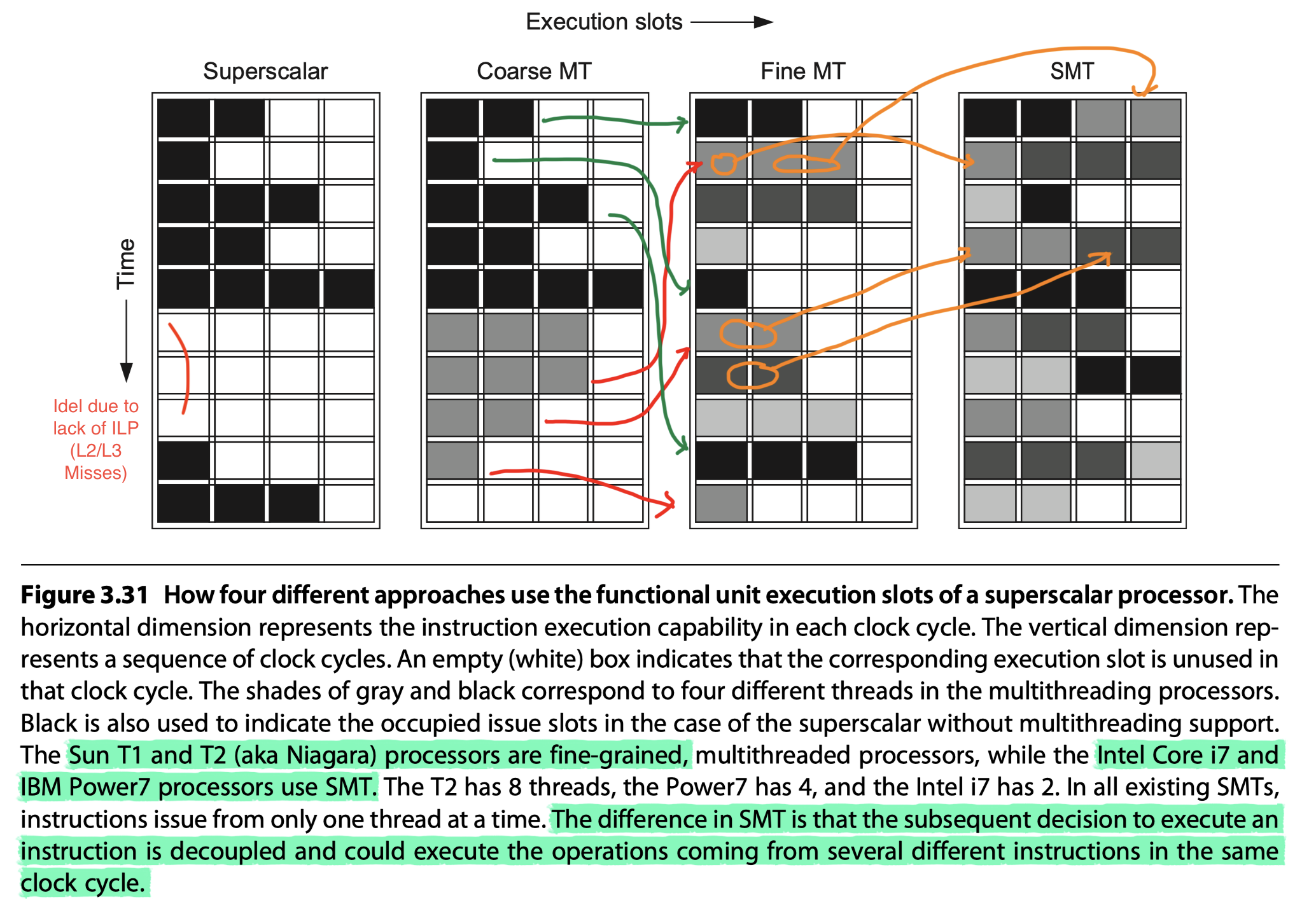
Fine-grained multithreading
- Switches between threads on each clock cycle
- SPARC T1 ~ T5 processors (Originally made by Sun, now by Oracle and Fujitsu)
- Transaction processing and web services
- T1 : 8 cores per processor and 4 threads per core
- T5: 16 cores per processor and 128 threads per core
- T2-T5 : 4-8 processors
- NVIDA GPUs
-
Coarse-grained multithreading
- Switches threads only on costly stalls, such as level two or three cache misses
- Relieved need to have thread-switching
- Less likely to slow down a single thread
- Suffer from limited throughput, especially from short stalls
- Bubble before the new thread begins executing = Start-up overhead
- No major current processors
-
Simultaneous multithreading (SMT)
- The most common implementation of multithreading
- SMT = Implementation of fine-grained multithreading on top of a multiple-issue, dynamically scheduled processor
- Key insight: Register renaming and dynamic scheduling allow multiple instructions from independent threads to be executed without regard to the dependences among them
- In all existing SMTs, instructions issue from only one thread at a time. The difference in SMT is that the subsequent decision to execute an instruction is decoupled and could execute the operations coming from several different instructions in the same clock cycle.
-
Fine-grained multithreading
Effectiveness of Simultaneous Multithreading on Superscalar Processors
- How much performance can be gained by implementing SMT?
- The existing implementations of SMT in practice
- $\rightarrow$ only two to four contexts with fetching and issue from only one, and up to four issues per clock
- $\rightarrow$ modest gain only.
-
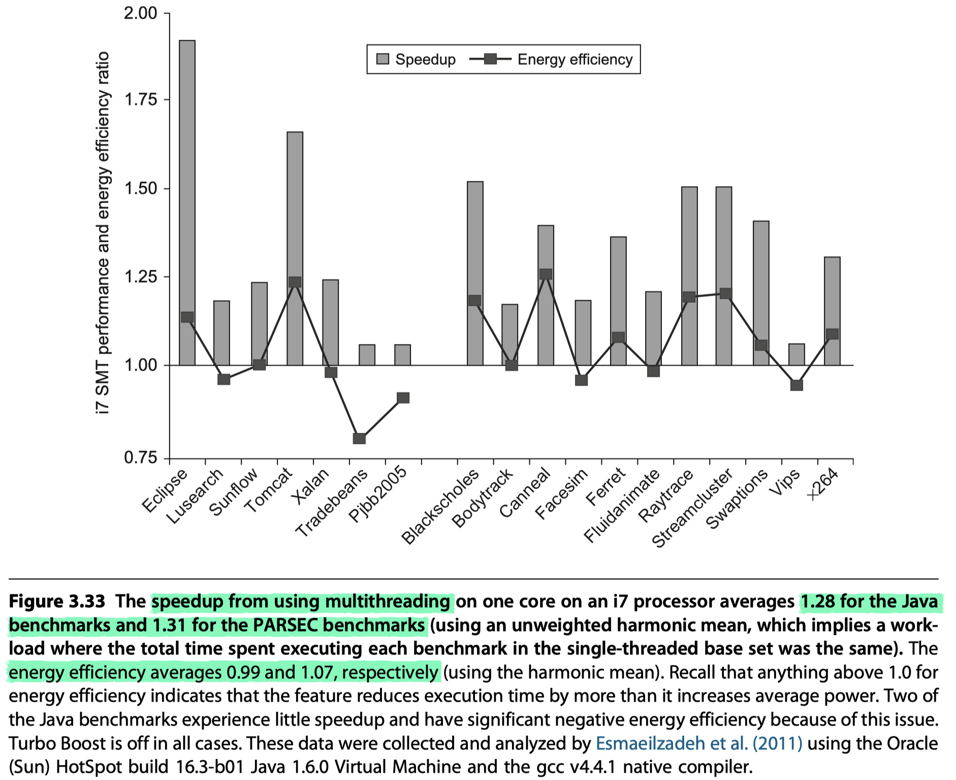
Dark Silicon and the End of Multicore Scaling
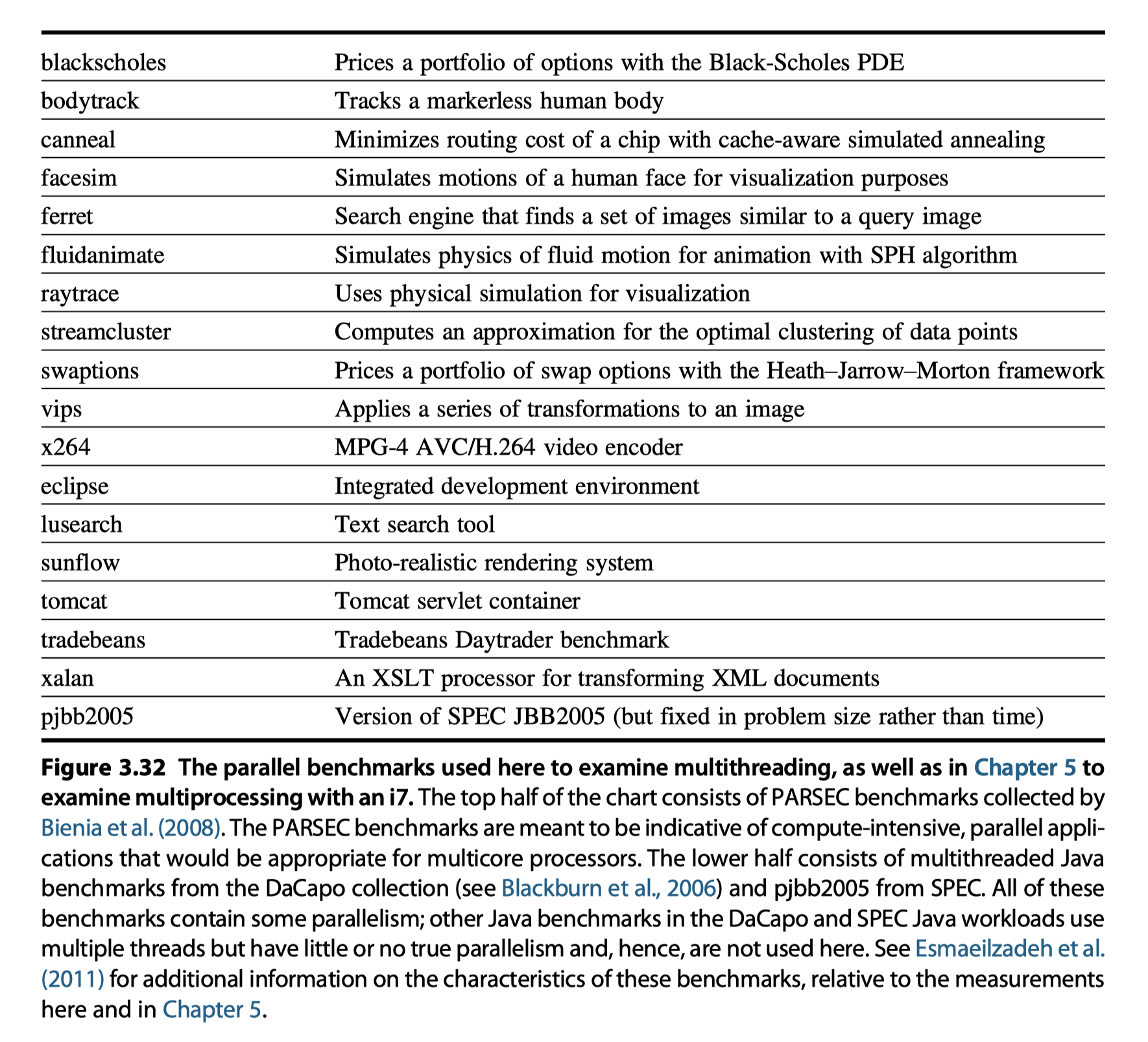
- Esmaeilzadeh et al. (2011)
- Examined performance and energy of using SMT in a single i7 920 core with two threads per core
Putting It All Together: The Intel Core i7 6700 and ARM Cortex-A53
The ARM Cortex-A53
-
A53
- Dual-issue (i.e. Allows the processor to issue two instructions per clock)
- Statically scheduled superscalar
- In-order pipeline
- Dynamic issue detection
- When the scoreboard-based issue logic indicates that the result from the first instruction is available, the second instruction can issue.
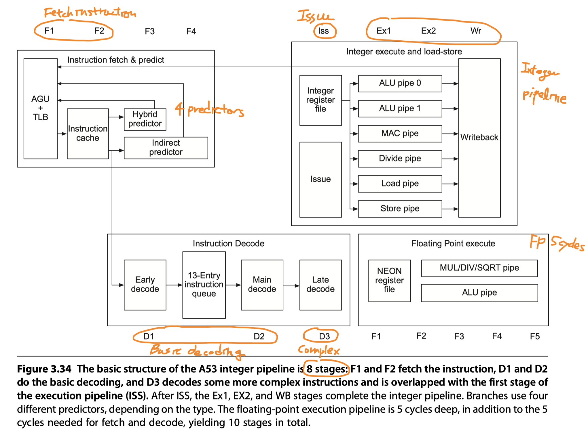
- Integer instructions
- 8 stages: F1, F2, D1, D2, D3/ISS, EX1, EX2, and WB
-
AGU = Address generation unit
- Produces next PC either
- By Incrementing the last PC or
- From one of four predictors
-
Predictors
- A single-entry branch target cache
- Containing two instruction cache fetches (= The next two instructions following the branch)
- Check the target cache during the 1st fetch cycle, if hit, the next two instructions are supplied
- No delay if hit and correct prediction
- A 3072-entry hybrid predictor
- Used if the branch target cache is missed
- Operating during F3
- Incur 2-cycle delay
- A 256 entry indirect branch predictor
- Operating during F4
- Incur 3-cycle delay
- An 8-deep return stack
- Operating during F4
- Incur 3-cycle delay
- A single-entry branch target cache
- Produces next PC either
- Branch decision
- Made in ALU pipe0 $\rightarrow$ Branch misprediction penalty = 8 cycles
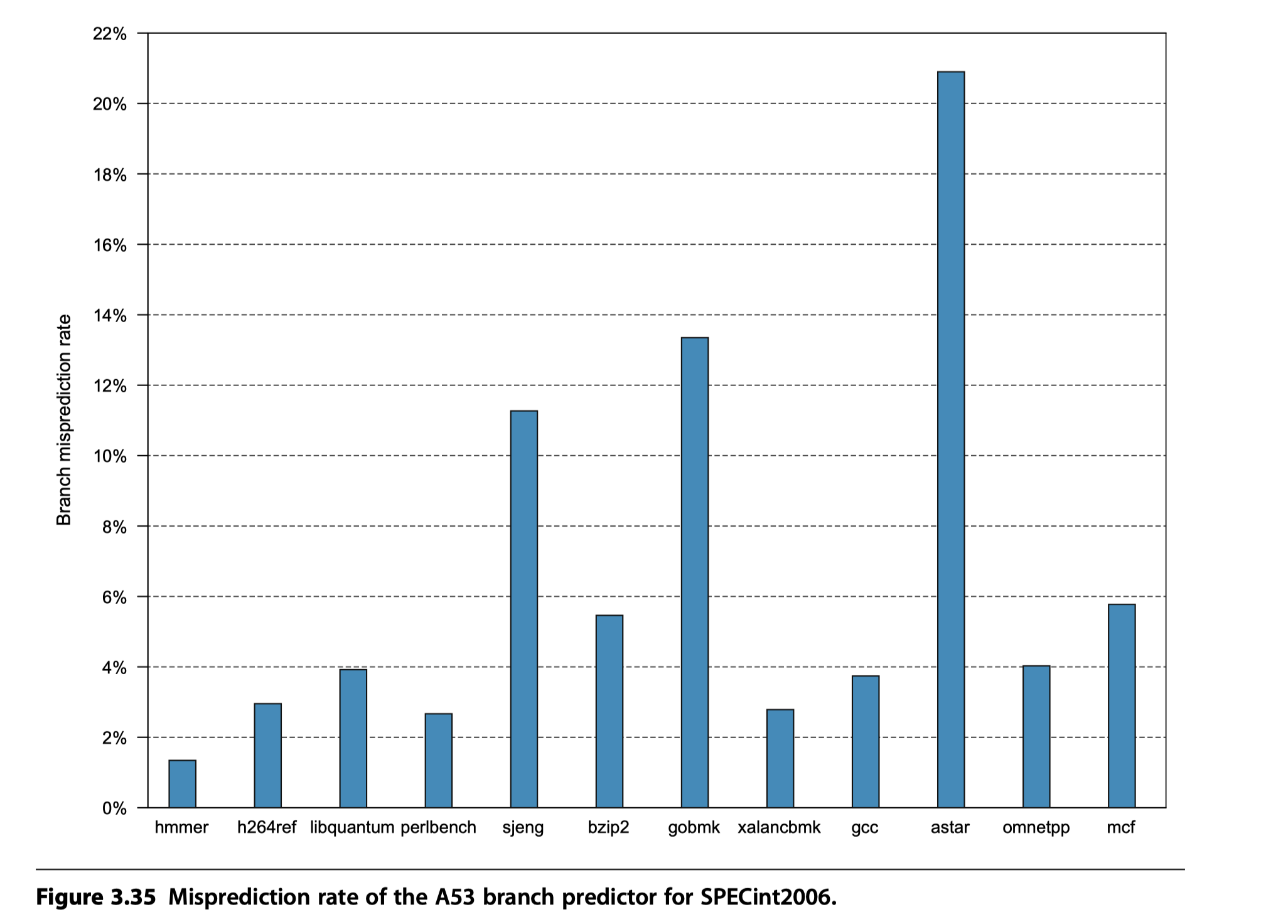
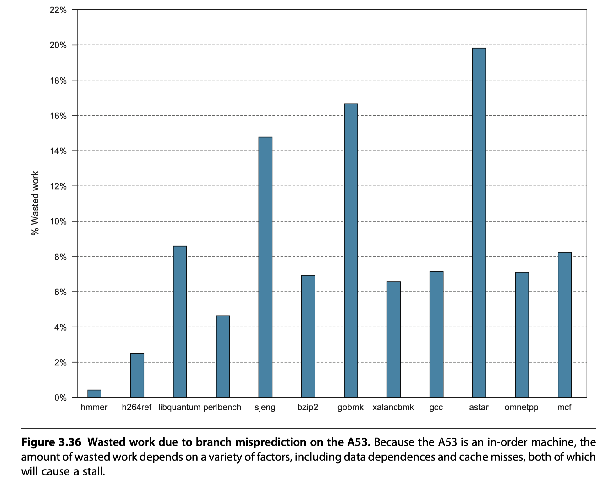
Performance of the A53 Pipeline
- Ideal CPI = 0.5
- Potential sources of pipeline stall
-
Functional hazards
- Two adjacent instructions selected for issue simultaneously use the same functional pipeline
- Compiler’s role to avoid this hazards
-
Data hazards
- Detected early
- Compiler’s role to avoid this hazards
-
Control hazard
- Arise only by misprediction
-
Functional hazards
- Memory hierarchy stalls
- TLB misses
- Cache miss
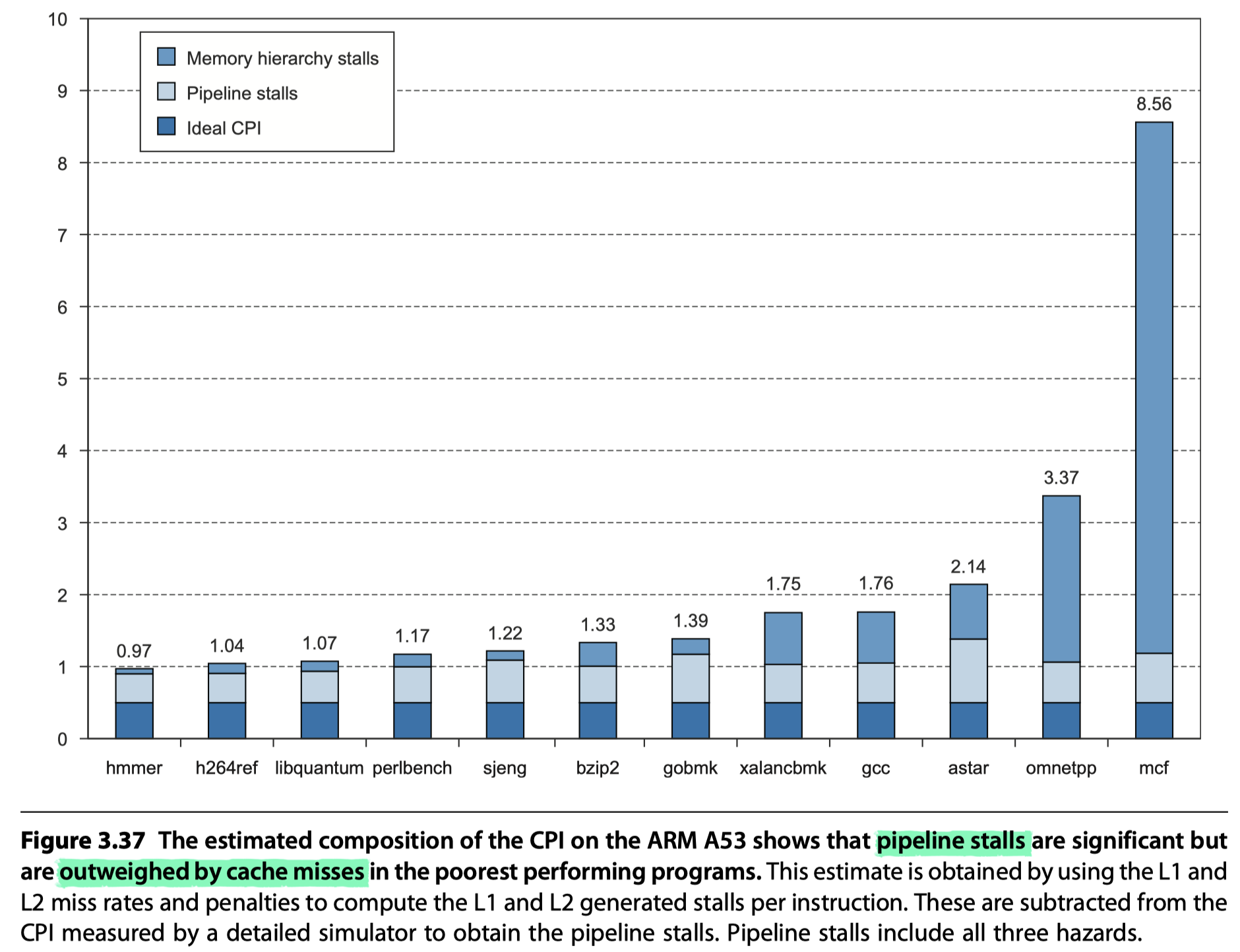
- Summary
- Shallow pipeline
- Reasonably aggressive branch predictor $\rightarrow$ Modest pipeline losses
- Achieve high clock rates at modest power consumption
- A53’s power ~ 1/200 power for a quad core i7 processor!!
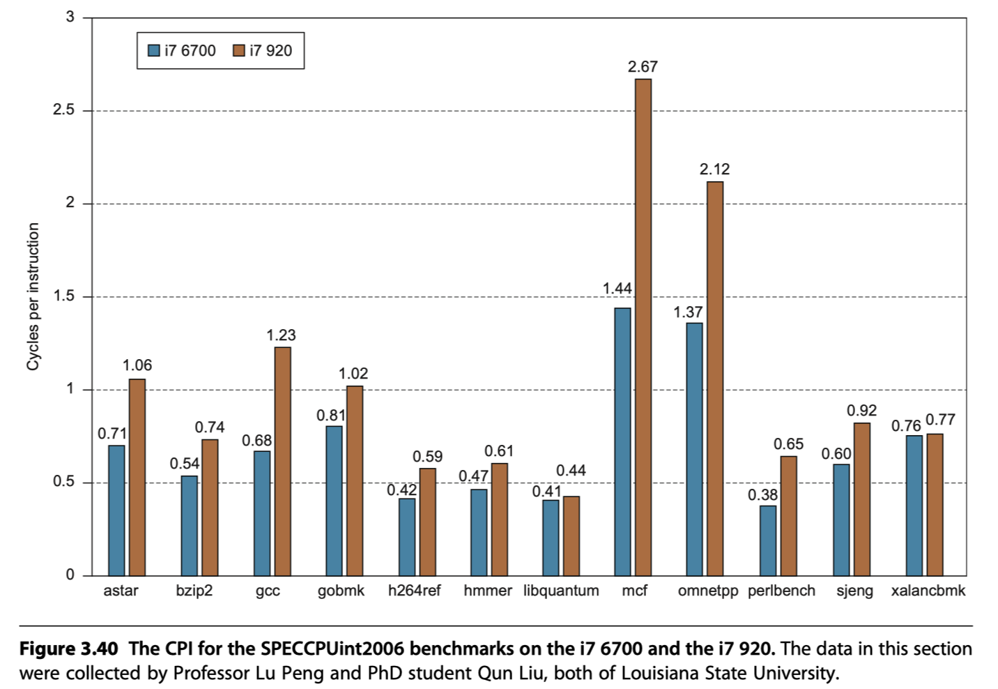
The Intel Core i7
-
Aggressive out-of-order speculative microarchitecture with deep pipelines
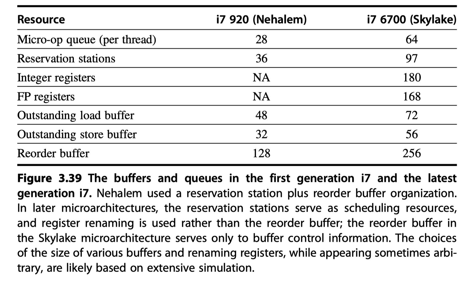
- i7 generations
- The first i7 in 2008
- Reservations stations + Reorder buffers
- Successive generations?
- Similar structure with enhanced performance by …
- Changing cache strategies (e.g., the aggressiveness of prefetching)
- Increasing memory bandwidth
- Expanding the number of instructions in flight
- Enhancing branch prediction
- Improving graphics support
- i7-6700 = The sixth generation
- Use explicit register renaming!
- With the reservations stations acting as functional unit queues and
- The reorder buffer simply tracking control information.
- The first i7 in 2008
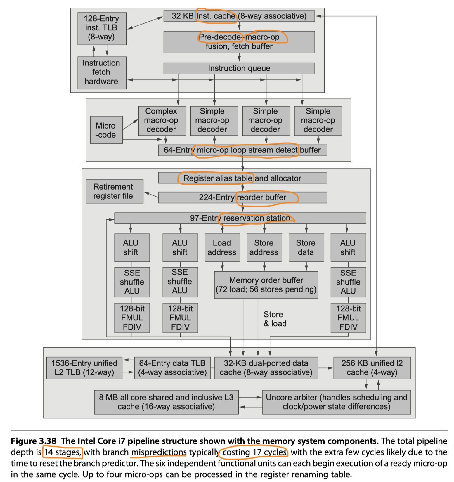
- i7 Pipeline
-
Instruction fetch :
- Multilevel branch predictor
- Return address stack
- Misprediction penalty = 17 cycles
- Fetch 16 bytes from the instruction cache using the predicted address
-
Macro-op fusion in a predecode instruction buffer
- Combine multiple instructions
- Issue and dispatch as one instruction (8-10% performance improvement for integer programs, not for floating point)
-
Micro-op decode
- x86 instructions $\rightarrow$ Translated into micro-ops
- Micro-ops = Simple RISC-V like instructions, directly executed by the pipeline
- Since 1997, Pentium Pro
- Four micro-ops every cycle
- Placed in the 64-entry micro-op buffer
-
Loop stream detection and microfusion in the micro-op buffer
- Loop stream detection: Find a loop comprised of a small sequence, directly issue the micro-ops from the buffer
- Micro-fusion: Combines instruction pairs (eg. ALU + a dependent store) to increase the usage of the buffer
- Basic instruction issue
- Look up the register location in the register table
- Rename the registers
- Allocate a reorder buffer entry
- Fetching results from registers or reorder buffer
- Send the micro-ops to the reservation stations
- A centralized reservation station shared by six function units
- Execute micro-ops, send the results to a reservation station or to the register retirement unit
- Instructions at the head of ROB $\rightarrow$ Marked as completed $\rightarrow$ Pending writes in the register retirement unit are executed
-
Instruction fetch :
i7 Performance

Reference
- Chapter 3 in Computer Architecture A Quantitative Approach (6th) by Hennessy and Patterson (2017)
- Notebook: Computer Architecture Quantitive Approach
Notes Mentioning This Note
Table of Contents
- Instruction-Level Parallelism and Its Exploitation
- Instruction-Level Parallelism: Concepts and Challenges
- Basic Compiler Techniques for Exposing ILP
- Reducing Branch Costs With Advanced Branch Prediction
- Overcoming Data Hazards With Dynamic Scheduling
- Dynamic Scheduling: Examples and the Algorithm
- Hardware-Based Speculation
- Exploiting ILP Using Multiple Issue and Static Scheduling
- Exploiting ILP Using Dynamic Scheduling, Multiple Issue, and Speculation
- Advanced Techniques for Instruction Delivery and Speculation
- Cross-Cutting Issues
- Multithreading: Exploiting Thread-Level Parallelism to Improve Uniprocessor Throughput
- Putting It All Together: The Intel Core i7 6700 and ARM Cortex-A53
- Reference